Accelerating Large-Model Inference: Engineering Practice from Hidden-State Extraction to DSpark Speculative Decoding

The core bottleneck of autoregressive generation in large models is well known—each step produces only a single token, each step requires moving all parameters from GPU memory to the compute units, and vast GPU compute capacity sits idle. Speculative decoding breaks through this bottleneck with a "small model drafts, large model verifies" paradigm, yet engineering tensions—insufficient draft quality, prohibitive hidden-state extraction costs, and incomplete cluster deployment pipelines—make real-world deployment far more complex than algorithm papers suggest.

This article dissects the end-to-end pipeline from Drafter training to native vLLM deployment, centering on the Speculators library and the DSpark algorithm. On the algorithm side, we examine how DSpark uses a Markov Head to trade less than 1.3% latency overhead for an 18–30% gain in acceptance length. On the engineering side, we explore how online hidden-state extraction reuses the KVConnector pipeline and how Mooncake Store closes the last mile of cross-node transfer.

Target audience: Backend or AI systems engineers familiar with large-model inference fundamentals who want a deeper understanding of speculative decoding internals and engineering optimizations.

Prerequisites:

• Familiarity with the basic principles of autoregressive generation in large models
• Working knowledge of inference engines such as vLLM
• A basic understanding of speculative decoding

Reading objectives:

1. Understand the decisive role acceptance length plays in the speedup ratio of speculative decoding
2. Master how DSpark uses a Markov Head to correct parallel generation
3. Learn the engineering ingenuity behind online hidden-state extraction that reuses KVConnector
4. Recognize the critical role of Mooncake Store in cross-node data transfer

---

1. The Engineering Value and Core Tensions of Speculative Decoding

Producing Multiple Tokens in a Single Forward Pass

The core idea of speculative decoding can be decomposed into three steps:

Phase	Role	Action	Key property
Propose	Lightweight Drafter (draft model)	Rapidly generate \(k\) candidate tokens	Can be autoregressive (e.g., EAGLE-3) or parallel (e.g., DFlash / DSpark)
Verify	Target (the large model)	Score all \(k\) positions in a single forward pass	Requires only 1 full forward pass; cost ≈ generating 1 token
Commit	Rejection Sampling	Accept the longest correct prefix; Target resamples at the first disagreement position	Lossless—the Target's output distribution is identical to that without speculative decoding

"Lossless" is the fundamental advantage that distinguishes speculative decoding from conventional acceleration techniques such as quantization and pruning: it does not alter the large model's output quality and gains speed purely by reducing the number of forward passes.

Illustration: Committing Multiple Tokens in a Single Verification

The figure below illustrates the complete "propose–verify–commit" process in speculative decoding, clarifying the data flow and decision logic at each phase.

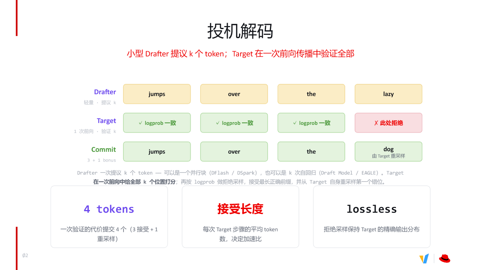Figure: The propose–verify–commit flow of speculative decoding. Source: presentation slides, page 3

Breaking down the key elements in the figure:

1. Drafter proposes 4 tokens: The draft model produces the candidate sequence jumps over the lazy in one shot.
2. Target verifies in a single forward pass: The large model receives all 4 candidates and computes the log probability at each position within one forward pass.
3. First 3 accepted: For jumps, over, and the, the Target's confidence is no lower than the Drafter's, so rejection sampling accepts them.
4. 4th rejected: lazy has an insufficiently high log probability according to the Target and is rejected.
5. Resampling yields a bonus token: At the rejected position, the Target resamples from its own distribution, producing dog. This token comes from the logits already computed in the current forward pass—no extra cost.
6. 4 tokens committed in total: 3 accepted + 1 resampled = a net gain of 4 tokens per Target step.

Acceptance Length: The Primary Determinant of Speedup

The entire causal chain can be condensed as follows:

Drafter quickly proposes k tokens
  → Target verifies all k positions in a single forward pass
    → Verification cost ≈ cost of generating 1 token
      → Net yield = acceptance length α (average accepted prefix length + 1 bonus)
        → Effective throughput improvement ≈ α×

The critical variable here is acceptance length—the average number of tokens produced per Target step. If the Drafter's guesses are inaccurate and frequently rejected, acceptance length approaches 1, speculative decoding degenerates into plain autoregressive generation, and the extra Drafter runs simply waste compute.

A minimal example illustrates this: suppose the input context is The and the Drafter proposes 3 tokens:

Step	Drafter proposal	Target verdict	Result
Position 1	lazy	✓ Accept	Retain
Position 2	dog	✓ Accept	Retain
Position 3	runs	✗ Reject	Target resamples → sat

One Target forward pass yields a net of 3 tokens (lazy dog sat), an effective speedup of roughly 3×.

Speedup Boundaries

According to engineering measurements shared in the talk, end-to-end speedups typically observed on vLLM (an open-source large-model inference and serving engine) fall in the range of 3–5×, depending on the algorithm and workload. However, speculative decoding has a hard boundary:

When the inference engine is compute-bound, speculative decoding provides no benefit and instead consumes additional compute.

The reason is straightforward: speculative decoding fundamentally trades surplus compute for fewer memory-transfer rounds. Once request concurrency is high enough to saturate GPU compute, no surplus remains. In this regime, it is advisable to dynamically disable speculative decoding and reserve all compute resources for the Target itself.

Summary: Speculative decoding losslessly widens the single-token-per-step bottleneck to multiple tokens per step, with the speedup determined by acceptance length. The next core question is: how do we train a more accurate Drafter to push acceptance length higher?

---

2. The Evolution of Modern Drafters: From Text to Hidden States

Why Early Approaches Had Limited Acceptance Rates

Early speculative decoding took a straightforward approach: use a smaller model from the same family as the draft—both receive the same natural-language text; the small model guesses first, and the large model verifies. Although the two models read the same prompt, their internal "depth of understanding" differs enormously. The small model predicts the next token with limited parameters, whereas the large model's predictions emerge from rich semantics distilled through dozens of Transformer layers. Under a text-only input regime, the output-distribution gap between the two is difficult to bridge, keeping the acceptance rate (the probability of confirmation at each position) stubbornly low and acceptance length correspondingly constrained.

The Key Turning Point: Letting the Drafter Peek at the Target's Internal Representations

The breakthrough began with a core insight—rather than forcing the Drafter to "understand" the prompt from scratch via raw text, feed it the intermediate results the Target model produces during the prefill phase.

This requires defining a key concept: hidden states, i.e., the intermediate activation values at each Transformer layer. For every token sequence the Target model processes, each layer outputs a set of vectors encoding that layer's semantic understanding of the input text—the deeper the layer, the higher the level of abstraction. Extracting hidden states from selected layers and providing them as Drafter input is tantamount to letting the small model make predictions while standing on the large model's semantic foundation, rather than reasoning from zero.

Architecture: How the Verifier and Draft Model Collaborate

The figure below shows how the Target (labeled "Verifier" in the diagram) passes multi-layer activations to the Draft model—an architectural foundation essential for understanding subsequent sections.

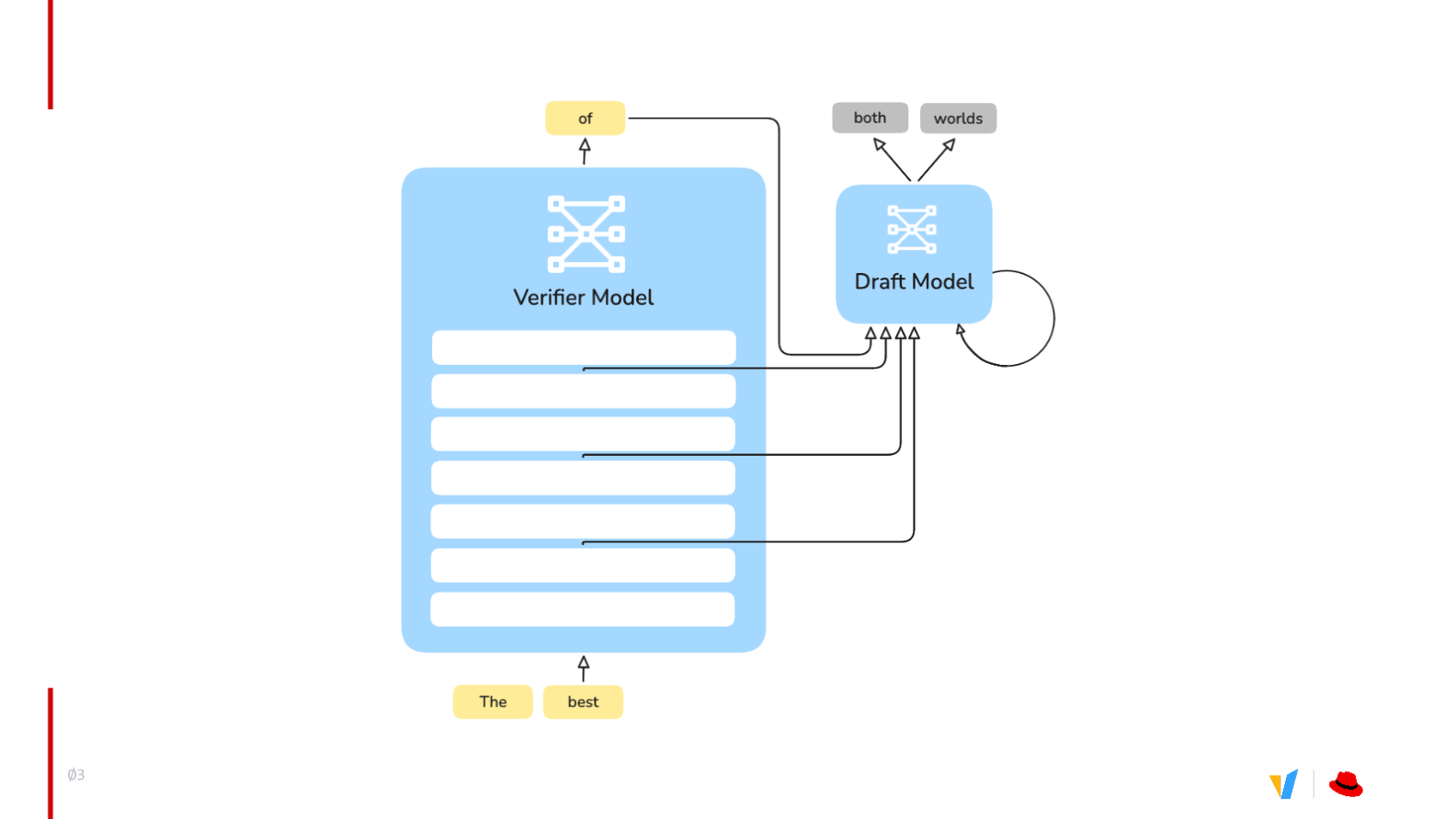Figure: Left—Verifier (Target) model; right—Draft model. Arrows indicate hidden-state transfer paths. Source: presentation slides, page 4

The figure contains two core components and one critical data path:

Component	Role	Characteristics
Verifier Model (left)	Receives raw tokens, executes a full forward pass, outputs predictions, and verifies drafts	Many layers, large parameter count
Draft Model (right)	Receives hidden states, rapidly generates multiple candidate tokens	Few layers (3–5), extremely fast inference

The data flow proceeds as follows: ① The Verifier receives input tokens; ② Hidden states are extracted from multiple layers of the Verifier and passed to the Draft model; ③ The Draft model outputs candidate tokens based on these states; ④ The Verifier also generates its own predictions and compares them token-by-token against the draft.

Contrasting the two input paths makes the difference clearest:

• Text-only path: Same prompt → small model understands independently → lacks the large model's intermediate reasoning cues → large output-distribution gap → low acceptance rate
• Hidden-state path: Target prefill produces multi-layer activations → Drafter obtains intermediate semantic representations → output distribution closely tracks the Target → acceptance rate improves → acceptance length grows

Layer-Extraction Strategies Across Algorithms

Algorithm	Layers extracted	Notes
EAGLE-3 (a classic autoregressive speculative decoding algorithm)	1 layer	Simplest structure, lowest overhead
DFlash / DSpark	3–5 layers	Multi-layer fusion, richer semantic information

More layers provide richer internal information from the Target but also incur greater activation transfer and storage costs. Three to five layers is the common choice for current high-performance Drafters, striking a practical balance between information richness and engineering overhead.

Summary: Switching from natural-language input to hidden-state input marks the watershed between "text-level imitation" and "representation-level learning" in speculative decoding. Building on this foundation, DSpark introduces a more refined architecture for producing higher-quality parallel drafts from these hidden states.

---

3. The DSpark Algorithm: Parallel Backbone with Markov Correction

Why Parallel Generation Can Produce Gibberish

The core guarantee of autoregressive generation is that each token can see every already-determined token to its left. Once generation is switched to parallel mode—producing multiple positions in a single forward pass—positions are mutually unaware of each other's predictions, and the conditional dependency between tokens breaks.

A minimal example: the user says "thank you," and reasonable replies include both "no problem" and "of course." If an autoregressive model outputs "of" at the first position, the second position will necessarily choose "course." In parallel generation, however, the first position selects "of" while the second independently selects "problem," producing "of problem"—the output degenerates into a meaningless combination. This is precisely the core bottleneck facing DFlash (a parallel speculative decoding algorithm based on non-causal mask tokens).

DSpark (a speculative decoding algorithm that combines a DFlash-style parallel backbone with a Markov Head for modeling intra-block dependencies) is designed with the goal of retaining DFlash's parallel throughput while restoring intra-block coherence at minimal cost.

Panoramic View of the DSpark Decoding Loop

The figure below provides a complete view of the three phases in each DSpark decoding round, showing how the parallel backbone, Markov correction, and confidence scheduling work in concert.

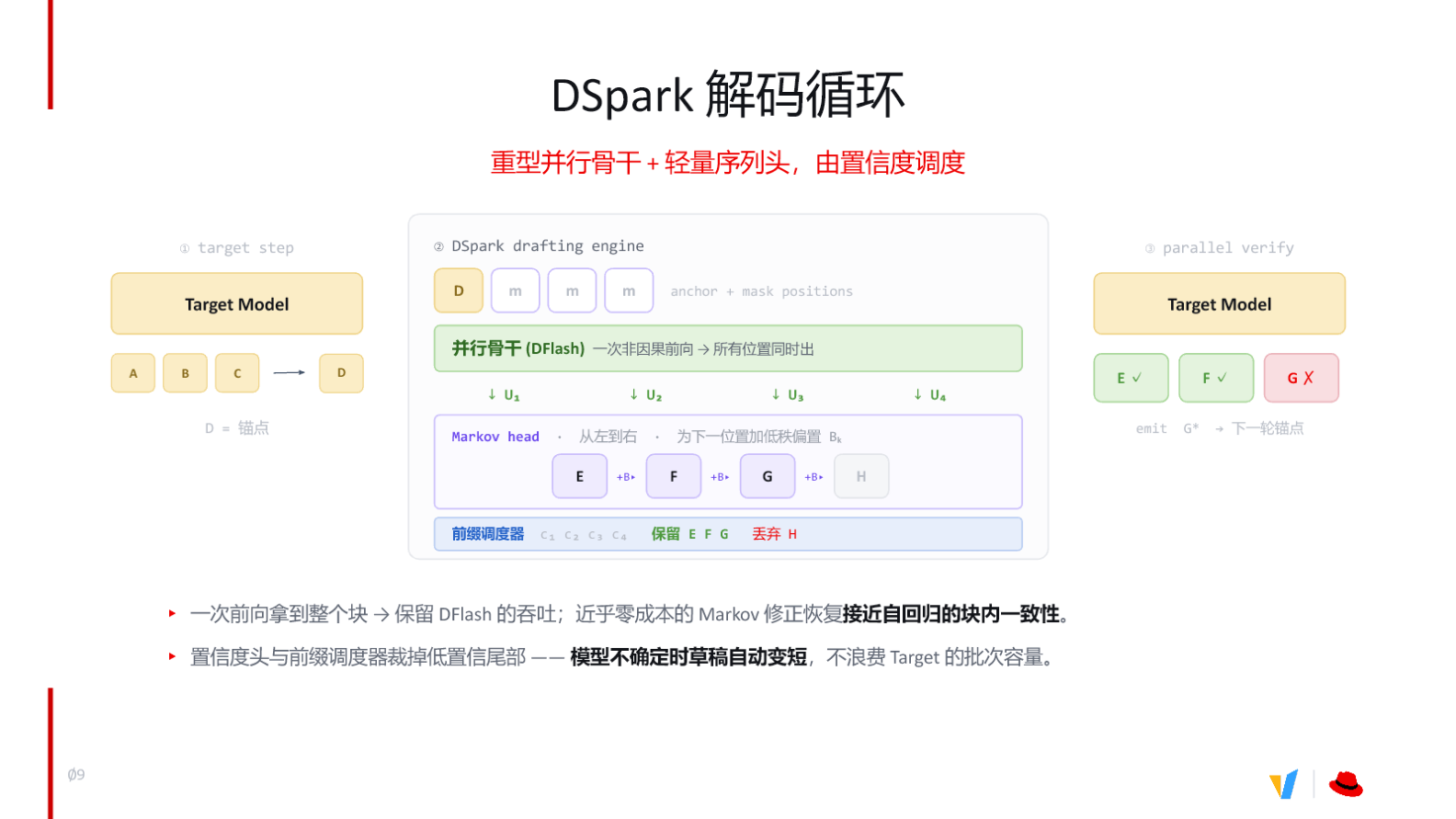Figure: The three-phase DSpark decoding loop. Source: presentation slides, page 10

① Target Step: Establishing the Anchor

The Target model performs one autoregressive forward pass, outputting the next token after the end of the accepted sequence, denoted D. D serves as the anchor for the current draft round—the left-boundary condition for subsequent parallel positions.

② DSpark Drafting Engine: Parallel Backbone + Markov Correction + Prefix Scheduling

This step is the heart of DSpark and consists of three internal layers:

Layer	Component	Input	Output	Cost
1	Parallel backbone (DFlash)	Anchor D + mask positions	Logits U₁–U₄ at all positions	One non-causal forward pass
2	Markov Head	U₁–U₄	Corrected token sequence E, F, G, H	Low-rank bias, near-zero cost
3	Prefix scheduler	Confidence scores c₁–c₄	Retain high-confidence prefix; truncate low-confidence tail	Threshold comparison only

Parallel backbone: Anchor D and several mask positions are fed into DFlash, which performs one non-causal forward pass to simultaneously obtain logits U₁–U₄ at four positions. Throughput is identical to vanilla DFlash.

Markov Head (a lightweight sequence head for correcting token dependency in parallel generation): A low-rank bias is applied sequentially from left to right across U₁–U₄. Specifically, the logits at position k+1 are augmented with a bias term determined by the token already selected at position k—E is corrected to yield F, F is corrected to yield G, and so on. The Markov Head is essentially a lightweight affinity matrix that learns token-to-token continuation probabilities; because the bias matrix is low-rank, the added latency is negligible.

Prefix scheduler: Each position simultaneously outputs a confidence score. The scheduler scans from left to right; as soon as a score falls below the threshold, that position and everything to its right are truncated. This ensures that drafts automatically shorten when the model is uncertain, preventing low-quality tokens from entering the Target's verification batch and wasting capacity.

③ Parallel Verify: Verification and Emission

The Target model performs one parallel verification over the retained draft tokens. Accepted tokens are committed directly; the first rejected position is resampled by the Target, producing a corrected token that becomes the anchor for the next round, and the loop restarts.

Causal Chain

Pure parallel generation → inter-token dependency breaks → output coherence degrades
  → Introduce Markov Head (low-rank bias, left-to-right positional correction)
    → Intra-block conditional dependencies restored → acceptance rate recovers
      → Add confidence head → prefix scheduler truncates low-confidence tail
        → Draft length becomes adaptive → Target verification overhead further reduced

Boundaries and Current Status

The Markov Head and the confidence head are two independent mechanisms that can be enabled individually or in combination. On the training side, both are supported in Speculators (a speculative decoding library covering training, conversion, and vLLM deployment). On the inference side, however, inference support for the confidence head is not yet fully ready in vLLM, and related work is ongoing. Consequently, current production deployments rely primarily on Markov Head correction to improve acceptance rates; the practical benefits of confidence scheduling remain to be validated on the engineering side.

---

4. DSpark Performance Validation and Boundary Conditions

Offline Evaluation Setup

To fairly compare EAGLE-3 (autoregressive drafting), DFlash (non-causal parallel drafting), and DSpark (parallel backbone + Markov Head), evaluation was conducted under the following controlled conditions:

Dimension	Value
Target model	Qwen3-14B
Sampling temperature	1.0
Draft mode	Chained drafting
Confidence scheduler	Disabled
Block-length range	4 → 16
Batch size	128

A temperature of 1.0 means maximum sampling randomness, raising the bar for draft-model prediction accuracy. Disabling the confidence scheduler eliminates the confound of adaptive pruning, making the comparison a purer reflection of draft quality itself.

Benchmark Data at a Glance

The figure below presents acceptance-length comparisons of the three algorithms across five representative tasks—the core evidence for judging the practical benefit of the Markov Head.

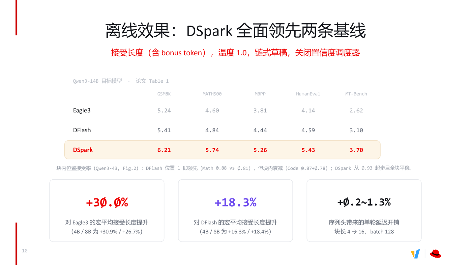Figure: Offline comparison—DSpark leads both baselines across all benchmarks. Source: presentation slides, page 11

The metric is acceptance length (including the bonus token), i.e., the number of tokens actually adopted after one Target verification. Higher values indicate more accurate drafts and greater speedup:

Dataset	EAGLE-3	DFlash	DSpark	DSpark lead over DFlash
GSM8K	5.24	5.41	6.21	+14.8%
MATH500	4.60	4.84	5.74	+18.6%
MBPP	3.81	4.44	5.26	+18.5%
HumanEval	4.14	4.59	5.43	+18.3%
MT-Bench	2.62	3.10	3.70	+19.4%

Macro-average summary below the table:

• +30.0% — DSpark's macro-average acceptance length improvement over EAGLE-3
• +18.3% — DSpark's macro-average improvement over DFlash
• +0.2–1.3% — Per-round latency overhead introduced by the Markov Head, increasing gradually as block length grows from 4 to 16, but never exceeding 1.3%

Why the Markov Head Is So Efficient

1. Missing intra-block dependencies → DFlash accuracy decay. DFlash uses a non-causal mask to generate an entire block of tokens in parallel; positions within the block cannot see each other. Per-position acceptance-rate data shows that on math tasks, DFlash decays from approximately 0.88 at the first position to roughly 0.78 at the block tail.
2. Markov Head injects low-rank bias → intra-block accuracy recovery. A low-rank bias is applied left to right at each successive position, correcting the independence-assumption error inherent in parallel generation. Under the same metric, DSpark starts at approximately 0.93 and remains stable across the entire block.
3. Per-position acceptance-rate gains → acceptance-length gains. Acceptance length is fundamentally determined by the product of per-position acceptance rates: a few extra percentage points at each position can compound into 18–30% overall growth.
4. Low-rank structure → minimal latency overhead. The sequence head's parameter count is far smaller than that of the parallel backbone; the additional computation accounts for only 0.2–1.3% of per-round inference time. Paying less than 1.3% in time yields an 18–30% gain in effective tokens.

Caveats and Applicability Boundaries

• Temperature sensitivity: The above results were obtained at temperature 1.0. At lower temperatures, draft hit rates are typically higher, and the relative magnitude of DSpark's advantage may change, but the presentation materials did not include low-temperature comparison data.
• Online end-to-end latency: This evaluation focuses on "acceptance length" as an offline metric. The actual end-to-end speedup in deployment is also influenced by scheduler efficiency, KV cache management, and other factors, requiring separate validation in an online environment.
• Additive effect of the confidence scheduler: The confidence scheduler was disabled for these benchmarks; the data reflects only the contribution of the Markov Head itself.

Summary: Under controlled offline conditions, DSpark achieves comprehensive leadership over both baselines at no more than 1.3% latency overhead. Training such a high-accuracy Drafter, however, first requires large-scale, high-quality hidden-state data—and this is the single greatest bottleneck in bringing the system to production.

---

5. The Training Data Bottleneck: The Bandwidth Wall of Offline Dumping

A Panoramic Comparison of the Two Paths

The knowledge distillation underlying the Drafter is built on intermediate-layer activations from the Target model, often spanning billions of tokens. Two fundamentally different engineering paths exist for obtaining these hidden states. The figure below presents a complete comparison of offline dumping versus online streaming—the starting point for understanding the engineering designs in the next two sections.

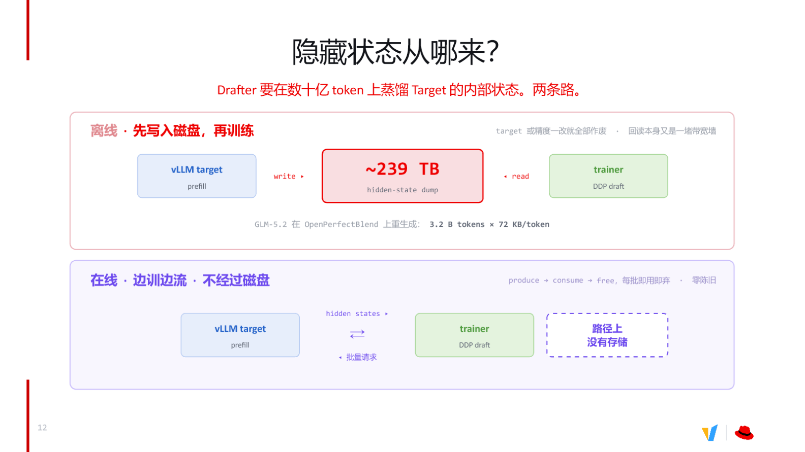Figure: The offline path requires disk as an intermediary; the online path directly produces → consumes → frees, with no persistent storage on the path. Source: presentation slides, page 13

The upper half of the figure shows the offline path: after vLLM Target completes prefill, hidden states are written to disk, producing massive hidden-state dump files; the trainer then reads these data back from disk. The lower half shows the online path: hidden states produced by vLLM Target are streamed directly to the trainer; once consumed, they are discarded—no persistent storage node exists on the path.

Three Fatal Bottlenecks of the Offline Path

Stage	Bottleneck description	Consequence
Write	The multi-layer hidden states per token are enormous; disk write bandwidth is saturated	Dumping time balloons from hours to days
Read-back	Training requires repeated reads from disk; disk I/O is far below GPU-memory bandwidth	Training GPUs idle for extended periods, utilization plummets
Staleness	Dumped data is strictly bound to the specific Target model weights and precision configuration	Any change in model or quantization scheme invalidates all data

A concrete data point conveys the scale: taking GLM-5.2 regeneration on the OpenPerfectBlend dataset as an example, the cumulative dump output is approximately 239 TB. This is infeasible in the vast majority of production environments.

The staleness issue is even more lethal: suppose a team spends several days completing the dump, and then the business side performs a parameter fine-tune or a quantization-precision adjustment on the Target model. Because hidden states are strictly coupled to Target weights, all previously dumped data instantly loses value, and the entire extraction pipeline must be rerun from scratch.

The Online Streaming Breakthrough

The core design of the online path is strikingly simple: the trainer issues batch requests to the vLLM Target; after the Target produces hidden states during the prefill phase, the activation data is consumed directly and then released—each batch is used once and discarded. The triple bottleneck of the offline approach is eliminated simultaneously—no massive storage required, no disk read-back latency, and activations always come from the current version of the Target model, inherently zero-staleness.

Regarding data volume requirements, training a Drafter for general-purpose scenarios typically calls for roughly 500,000 conversation samples (e.g., Magpie, UltraChat, etc.); for domain-specific fine-tuning, practical experience suggests that 30,000 to 70,000 samples can yield good acceleration gains (these are empirical values shared during the talk, not conclusions from rigorous experiments). Online streaming makes acquiring these data on demand a low-cost operation.

Conclusion: Offline dumping simultaneously hits walls on storage scale, read/write bandwidth, and data freshness. Online extraction is the practically viable choice—but it introduces a new engineering problem: how do we move hidden states out of the engine without intruding on vLLM's core logic?

---

6. The Online Extraction Mechanism: A Clever Disguise as KV

From "Building a Path" to "Borrowing a Path"

The most intuitive approach to online extraction is to build a dedicated pipeline inside the inference engine, but this means deeply intruding on vLLM's scheduling and memory-management logic—high engineering cost and prone to conflicts during upgrades. A better strategy is to reuse the engine's existing high-bandwidth paths.

The reasoning unfolds in four steps:

1. Building a new path requires rewriting scheduling, memory allocation, and concurrency control, incurring heavy maintenance burden.
2. vLLM already has a well-polished KVConnector transfer pipeline for KV Cache (the Key/Value tensors cached during attention computation).
3. KV Cache slots are organized as [Token, num_heads, head_size]; the auxiliary activation stack is also a three-dimensional tensor [T, L, H].
4. By mapping the layer axis L to num_heads and the hidden dimension H to head_size, the activation stack fits seamlessly into existing slots.

Dimension-Mapping Details

During the Target's forward pass, activation values are extracted from designated intermediate layers (e.g., layers 8, 23, 39, 55, 70) and stacked along the layer axis, yielding a tensor of shape [T, L, H]:

Symbol	Meaning	Corresponding KV-slot semantic
T	Number of tokens in the current batch	Token dimension—unchanged
L	Number of extracted layers (e.g., 5)	Treated as num_heads
H	Hidden-state dimension per layer	Treated as head_size

This mapping requires no reshape or transpose operations—the memory layout is natively consistent. The engine treats the stack as a set of "virtual attention heads," writes it directly into KV slots, and sends it out via KVConnector.

The figure below illustrates the specific mapping relationship and the data flow within the engine.

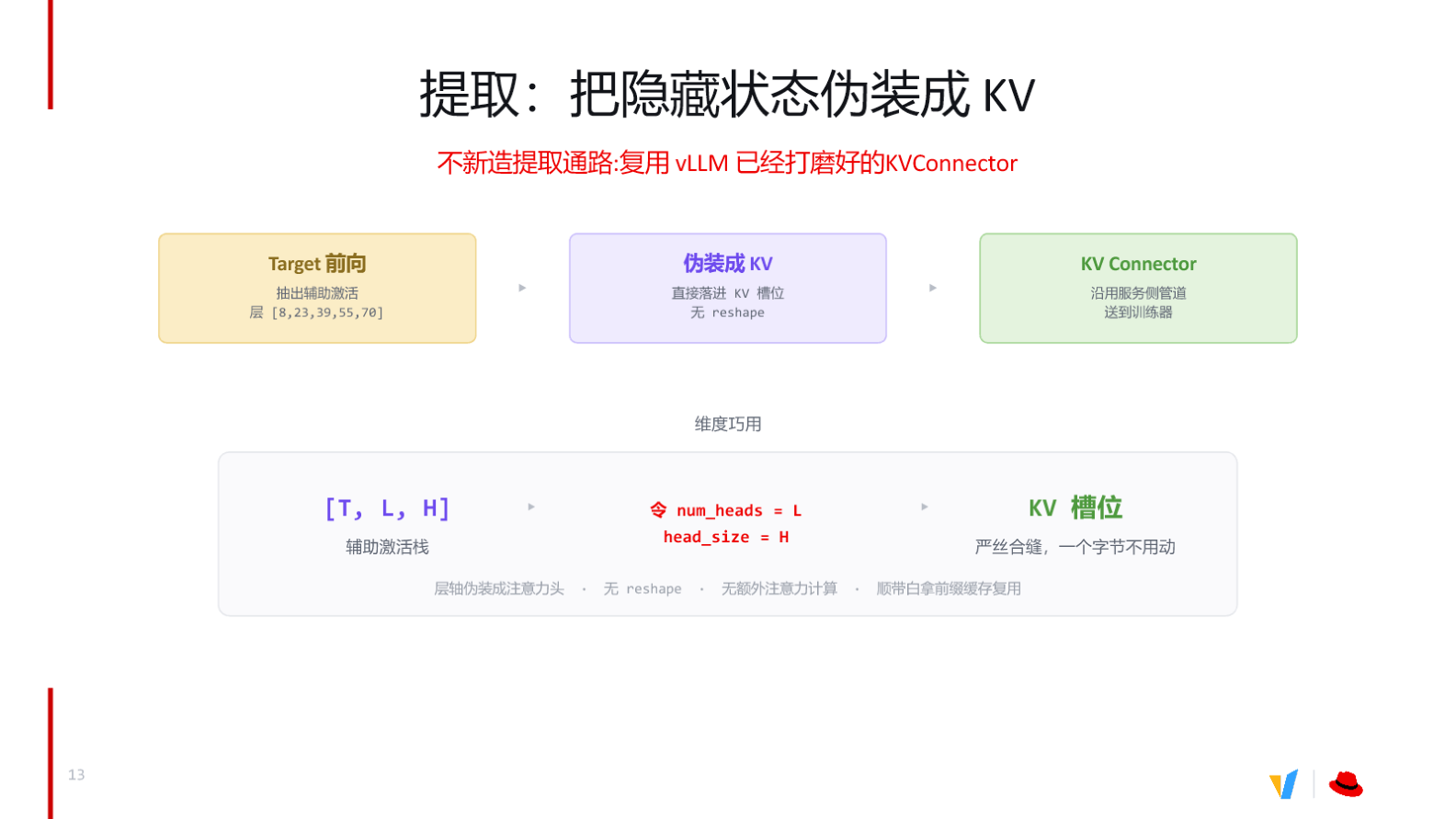Figure: Hidden-state extraction and the KV-disguise mechanism—the layer axis acts as num_heads, the hidden dimension acts as head_size, dropping directly into existing KV slots. Source: presentation slides, page 14

The figure depicts three stages from top to bottom:

• Target forward pass: Activations are extracted from five designated layers and stacked into the auxiliary activation stack [T, L, H].
• Disguised as KV: L is labeled num_heads and H is labeled head_size; the stack fits into KV Cache slots with no copy or reordering.
• Sent out via KVConnector: The existing serving-side transfer pipeline is reused to send the disguised "KV" to the trainer, additionally benefiting from prefix caching.

Minimal State Evolution

Assume 5 extracted layers, a hidden dimension of 4096, and a current batch of 32 tokens:

Original auxiliary activation stack shape: [32, 5, 4096]
Shape as seen by the engine:              [32, num_heads=5, head_size=4096]
→ Written directly into KV slots, zero-byte copy
→ Sent out by KVConnector via the standard KV transfer flow
→ Trainer receives and interprets under [T, L, H] semantics

Throughout this process, no additional attention computation is triggered, and the engine's KV Cache management logic is not modified.

Boundaries and Limitations

This approach presupposes that the KVConnector implementation requires the producer (Target inference process) and the consumer (trainer) to reside on the same node, sharing part of the memory region. When model scale is large enough that a single node cannot host both, or when training and inference must reside in separate node pools, this local shared-memory constraint becomes a bottleneck—which is the direct motivation for introducing a cross-node connector.

---

7. Cross-Node Transfer: Introducing Mooncake Store

The Transfer Dilemma of Pool-Separated Deployment

When the Target model reaches the scale of the Qwen3 (Qianwen large model series) family, GPU memory barely permits inference and training to coexist on the same machine. The engineering solution is pool separation: inference nodes focus exclusively on running online prefill while training nodes focus exclusively on consuming hidden states for gradient updates. Once pool separation is in place, cross-network transfer becomes unavoidable.

Four Hard Requirements

The talk explicitly enumerates four constraints that this transfer path must satisfy simultaneously:

#	Requirement	Practical reason
①	Cross-node, without assuming a shared file system	The producer pool and the trainer pool reside on different machines; many clusters lack a high-speed shared FS
②	Key-addressable	The producer does not know who will consume or when; neither side can address the other directly
③	One-sided read	Transfer operations must not occupy the producer's CPU—it is still serving online requests
④	Bounded + evictable	If the consumer goes offline and production speed exceeds consumption speed, it must be possible to stop writing and clean up

Requirement ④ is particularly critical: the speaker mentioned that during actual training, incidents had occurred where the consumer stopped working while the producer continued writing, eventually filling up disk.

Candidate Solutions Compared

The figure below lists four candidate solutions and how each meets the four requirements—the decision basis for choosing Mooncake Store.

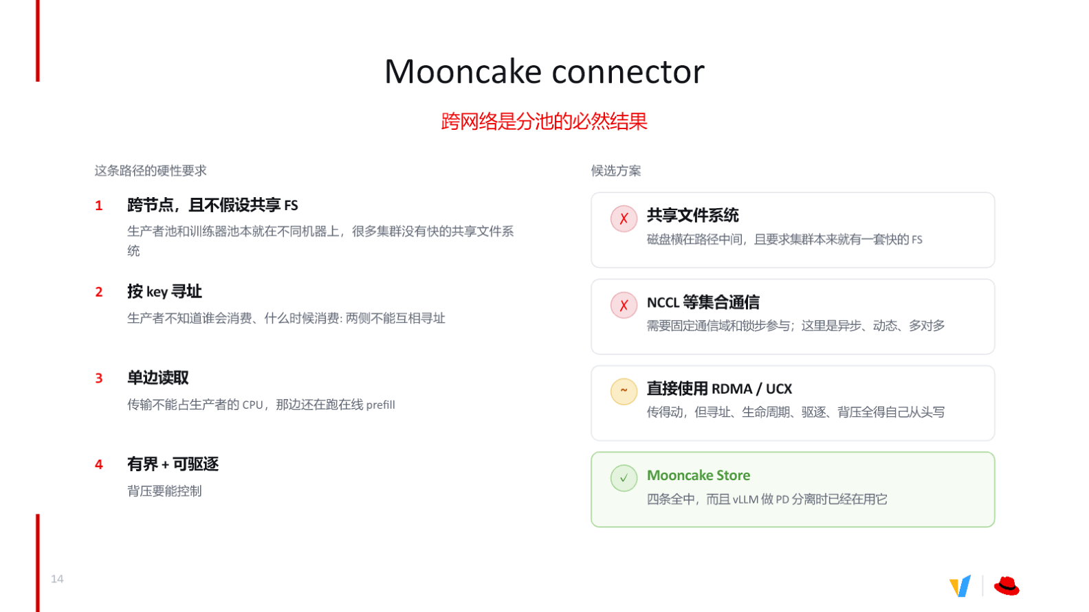Figure: Cross-network transfer candidate solutions and their satisfaction of the four requirements. Source: presentation slides, page 15

Analyzing each in turn:

• Shared file system ✗ — Disk I/O stands in the transfer path, and the solution depends on a pre-installed high-speed FS in the cluster, yielding poor generality.
• NCCL and other collective communication ✗ — Requires a fixed communication domain and lock-step participation; this scenario is asynchronous, dynamic, and many-to-many in topology—a complete mismatch.
• Direct RDMA / UCX ～ — Bandwidth is sufficient, but addressing, lifecycle management, eviction, and back-pressure strategies all need to be built from scratch, entailing substantial engineering effort.
• Mooncake Store ✓ — All four requirements are satisfied, and vLLM has already integrated this component for PD (Prefill-Decode) disaggregation, providing a relatively mature foundation.

How Mooncake Store Works

Mooncake (a cross-network connector/store) provides cross-node, key-addressable, one-sided-read key–value storage capability, purpose-built for high-speed transfer of intermediate tensors such as hidden states. Its core characteristics include: the writer only needs to put(key, tensor), the reader can proactively pull by key without involving the producer in scheduling, and it has built-in bounded buffering and TTL eviction mechanisms.

A minimal workflow:

1. The vLLM inference node, upon completing a prefill, writes the hidden states to the local Mooncake Store as (request_id, tensor) and immediately returns to process the next request—the CPU is not blocked by the transfer.
2. The trainer node uses the known request_id (key) to pull the corresponding tensor from Mooncake Store via RDMA one-sided read; the entire process does not interrupt any thread on the inference side.
3. If the trainer node fails to consume within the time limit, Mooncake Store automatically evicts expired data according to its TTL policy, preventing memory overflow.

Conclusion and boundaries: Mooncake Store closes the critical last mile for cluster-scale online extraction. Its applicability boundary lies in its dependence on RDMA network availability; the presentation materials did not provide specific bandwidth or latency benchmark data for cross-node transfer, so actual throughput must be assessed in conjunction with the cluster's network topology.

---

8. Speculators: An End-to-End, All-in-One Closed Loop

The Last-Mile Barrier

The preceding sections discussed DSpark's algorithmic design, online hidden-state extraction, and cross-node transfer. In actual production, however, engineers face yet another barrier: how can a trained Drafter run inside an inference engine with zero modifications? The traditional approach typically requires hand-writing model-loading logic, aligning configuration parameters, and maintaining format-conversion scripts—any misstep can cause accuracy or performance regression.

The Speculators library is designed precisely to eliminate this gap. It covers the full pipeline of data preparation → hidden-state extraction → model training → format conversion → inference deployment, with the core promise that: the Drafter checkpoint and config produced by training can be natively loaded and served by vLLM without any glue code. It supports online extraction, offline extraction, and hybrid modes, and also covers architectures such as MoE (Mixture of Experts) and VLM (Vision-Language Models).

How a Single config.json Drives vLLM

The figure below shows the key fields in the config.json exported by Speculators and vLLM's automatic detection flow—the core mechanism behind "zero glue."

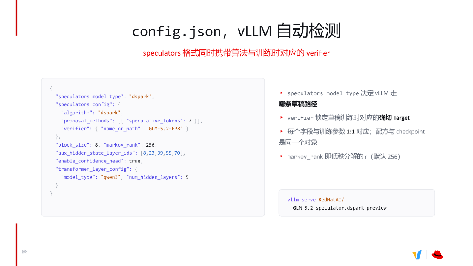Figure: Core fields of config.json and the vLLM automatic detection mechanism. Source: presentation slides, page 9

The JSON configuration in the figure contains the following key fields, each strictly corresponding to a training parameter:

Field	Example value	Purpose
speculators_model_type	"dspark"	Tells vLLM to select the DSpark drafting path
verifier	"GLM-5.2-FP8"	Locks in the Target model identifier used during training
markov_rank	256	Rank of the low-rank decomposition in the Markov Head; determines the parameter count for intra-block dependency correction
block_size	8	Token block size per draft generation round
aux_hidden_state_layer_ids	[8, 23, 39, 55, 70]	Layer indices from which the Drafter extracts hidden states in the Target
enable_confidence_head	true	Whether to enable the confidence head for early termination
transformer_layer_config	num_hidden_layers: 5	Number of Transformer layers and architecture type for the Drafter itself

The annotation on the right side of the figure explicitly states: The recipe and the checkpoint are the same object. The configuration file and weight files are bundled at release time, eliminating any risk of version drift.

Causal Chain: Why "Zero Glue" Is Achievable

1. Traditional pain point: Drafter training scripts and the inference engine each maintain their own parameter definitions; engineers must hand-write a conversion layer to map training formats to formats the engine can recognize. If parameter names, dimensions, or layer indices do not align, acceptance rates plummet or inference throws errors.
2. Speculators' solution: Upon training completion, a HuggingFace-compatible checkpoint directory is output directly, with config.json carrying the complete algorithm type and training hyperparameters. At startup, vLLM reads speculators_model_type and automatically routes to the corresponding draft-construction logic; all parameters are injected from the same config.
3. End result: Deployment requires only a single command—vllm serve <model_path>—and the engine assembles the complete speculative decoding inference graph according to the fields in the config.

Minimal Deployment Example

Suppose a DSpark Drafter targeting GLM-5.2-FP8 has been trained with Speculators and exported to the directory RedHatAI/GLM-5.2-speculator.dspark-preview. Deployment requires exactly one step:

vllm serve RedHatAI/GLM-5.2-speculator.dspark-preview

Upon reading speculators_model_type: "dspark", vLLM automatically initializes the Markov Head and parallel drafting backbone with markov_rank=256 and block_size=8. To adjust the rank of the low-rank decomposition, simply modify markov_rank before retraining; after training completes, the config naturally carries the new value, and the deployment command remains unchanged.

Boundary Conditions

Although Speculators drastically lowers the engineering barrier for speculative decoding, one rigid constraint exists: the Target model identified by the verifier field in config.json must be strictly identical to the Target used during training. If the production environment switches Target versions (e.g., from an FP8 quantized version to a BF16 full-precision version), the Drafter's hidden-state input distribution will shift, and acceptance rates may drop significantly—retraining or at least fine-tuning is then required. The presentation materials did not provide performance-degradation data for reusing a Drafter across Target versions.

---

Conclusions and Limitations

Core Conclusions

1. Acceptance length is the primary determinant of speculative decoding's speedup ratio. The more tokens accepted in a single Target verification, the greater the reduction in forward passes and the more pronounced the end-to-end throughput improvement.
2. Upgrading the input from text to hidden states is the key to modern Drafters achieving high acceptance rates. Extracting 3–5 layers of intermediate activations from the Target model for distillation training allows the Drafter to reuse the semantic reasoning the large model has already performed, significantly narrowing the output-distribution gap.
3. DSpark solves the intra-block coherence problem of parallel generation at minimal cost. The Markov Head applies low-rank bias corrections position by position from left to right. Under controlled conditions—Qwen3-14B, temperature 1.0, chained drafting, confidence scheduler disabled—DSpark achieves a 30.0% macro-average acceptance-length improvement over EAGLE-3 and an 18.3% improvement over DFlash, with per-round latency overhead of only 0.2–1.3%.
4. Offline dumping faces a triple bottleneck of storage (~239 TB scale), bandwidth, and data staleness. The online train-while-streaming approach completely eliminates persistent storage requirements through a use-once-and-discard data flow.
5. Online extraction reuses the KVConnector pipeline, disguising the hidden-state layer axis as the attention-head dimension, achieving a zero-copy, zero-reshape, high-cost-effectiveness engineering solution.
6. Mooncake Store closes the last mile for cross-node scenarios, satisfying all hard requirements of key-addressable, one-sided read, and bounded-with-eviction semantics.
7. The Speculators library provides an all-in-one solution. The checkpoint and config produced by training can be natively loaded by vLLM, eliminating glue code between training and deployment.

Explicit Limitations

• No benefit under compute-bound conditions. When the inference engine's GPU compute is already saturated, speculative decoding cannot trade compute for speed and instead incurs additional overhead; it should be dynamically disabled in this regime.
• Inference-side support for the confidence head is not yet fully ready. DSpark's confidence scheduler mechanism is still under development in vLLM; current production deployments rely primarily on Markov Head correction.
• Applicability conditions for performance data must be strictly preserved. The 30.0% and 18.3% improvement figures come from a specific setup—Qwen3-14B, temperature 1.0, chained drafting, confidence scheduler disabled, block length 4–16, batch size 128—and must be re-validated when generalizing to other models and parameters.
• The Drafter is strictly coupled to the Target. Once the Target model version or quantization scheme changes, the existing Drafter's acceptance rate may degrade significantly, necessitating retraining or fine-tuning.
• Mooncake Store depends on RDMA networking. The presentation materials did not provide specific bandwidth or latency benchmark data for cross-node transfer; actual throughput must be assessed in conjunction with the cluster's network topology.