GLM-5 Ascend Inference Optimization: A Systematic Dissection from Architectural Bottlenecks to End-to-End Performance

Source video: Bilibili BV1eoJJ6eEUv · Slides: GLM-5 Optimization

The engineering difficulty of deploying large language model inference often lies not in conquering any single technical challenge, but in the perpetual tug-of-war among latency, throughput, and memory. GLM-5, a large model employing a MoE (Mixture of Experts) architecture with a unique attention structure, pushes this tug-of-war to the extreme under long-sequence inference scenarios: computation explodes during the Prefill stage, KV Cache devours memory, and communication overhead dominates the Decode stage—no single-point optimization suffices to address the problem holistically.

This article is based on the inference optimization practice of GLM-5 on the Huawei Ascend platform. Following the causal chain of "metric definition → bottleneck identification → architectural decomposition → data compression → operator acceleration → end-to-end validation," it systematically dissects the complete path from analytical framework to engineering implementation.

Target audience: AI engineers and architects with a foundation in large models who are focused on inference performance optimization, compute deployment, and low-level acceleration mechanisms.

Prerequisites:

• Familiarity with the basic process of large language model inference (the two-stage Prefill and Decode pipeline).
• Knowledge of common distributed parallelism strategies (TP, DP, PP).
• A basic understanding of memory bandwidth, compute-bound tasks, and memory-bound tasks.

Reading objectives:

1. Master the core metrics of large model inference performance and their mutual constraints.
2. Understand the structural bottlenecks of GLM-5 in long-sequence scenarios.
3. Learn to design PD disaggregation and differentiated parallelism strategies based on compute and memory-access characteristics.
4. Understand the acceleration principles of quantization, graph mode, and fused operators on Ascend hardware.

---

1. Core Conflicts and Analytical Framework for Inference Optimization

Central question of this section: What should be done first in large model inference optimization? How do we establish a reusable analytical methodology?

When deploying GLM-5, the first question an engineer faces is not "how to optimize" but "what to optimize, and for whom." Optimization divorced from business objectives merely oscillates between latency and throughput. This section clarifies the constraint relationships among four core performance metrics and presents a four-step analytical methodology that provides the basis for all subsequent optimization decisions.

Four Core Metrics and Two Stage Types

Large model inference performance is characterized by four metrics:

Metric	Full Name	Determining Factor	Nature
TTFT	Time To First Token	Prefill stage processes the entire input prompt	Compute-bound; positively correlated with input length
TPOT	Time Per Output Token	Decode stage generates tokens one at a time	Memory-bound; constrained by bandwidth and memory
Throughput	Total tokens generated per unit time (TPS)	Overall system processing capacity	Generally increases with concurrency, but has an upper bound
Concurrency	Number of requests the system can serve simultaneously	HBM capacity ceiling	Directly constrained by KV Cache footprint

Prefill (the first inference stage, which processes the entire input sequence in one pass) and Decode (the generation stage, which outputs tokens one at a time) are fundamentally different in nature: the former is bottlenecked by compute, the latter by memory bandwidth. This means a single optimization technique can rarely improve both TTFT and TPOT simultaneously—before choosing an optimization direction, one must first know which end the business cares about more.

The Core Conflict: Latency and Throughput Cannot Be Maximized Simultaneously

A fundamental trade-off chain exists among the four metrics:

Increasing batch size / concurrency → throughput ↑, but per-request TTFT and TPOT also ↑; Pursuing ultra-low latency (small batch) → compute units are underutilized, throughput ↓, unit cost ↑.

The physical root of this trade-off chain lies in the sharing of three categories of resources:

1. Compute: As batch size increases, compute unit utilization improves, but per-request queuing and scheduling overhead also increases.
2. Bandwidth: During the Decode stage, multiple requests share HBM bandwidth; the higher the concurrency, the lower the effective bandwidth allocated to each request.
3. Memory: Weights, KV Cache (Key-Value Cache—the cached historical key-value pairs used during inference), and activations collectively occupy HBM. KV Cache grows linearly with the number of concurrent requests, directly determining the maximum concurrency the system can accommodate.

Memory is the master gate. No matter how powerful the compute or how large the bandwidth, once HBM is filled by weights and KV Cache, no new requests can be admitted. The SLO (Service Level Objective) sets an upper bound on batch size, while memory sets the ceiling; the actual usable value is the minimum of the two.

Four-Step Analytical Framework

When facing inference optimization for any model, the following four-step closed loop can be applied:

Step	Action	Key Input
① Define metrics and objectives	Establish business SLOs: input/output lengths, TTFT ceiling, TPOT ceiling, target throughput and concurrency	Product requirements document
② Identify bottlenecks	Distinguish Prefill / Decode; determine whether compute-bound or memory-bound; locate the chokepoint	Profiling data
③ Select strategies	Apply targeted remedies from parallelism combinations, quantization, PD disaggregation, graph mode, etc.	Hardware topology and framework capabilities
④ Validate quantitatively	Use measured TTFT / TPOT / throughput to verify against SLOs; iterate on parameters until targets are met	End-to-end benchmarks

When evaluating every optimization point, always ask three questions: Which bottleneck does it address? Which metric does it improve? What cost does it incur? If the answers are unclear, the optimization direction has not yet been aligned with business objectives.

Minimal Example: Deriving Batch Size from an SLO

Suppose the business requires TPOT < 50 ms, and single-card Decode takes 10 ms per step at batch=1. If TPOT scales approximately linearly with batch size (an idealized assumption for illustrative purposes):

\[\text{TPOT} \approx t_{\text{base}} \times B / B_0\]

where \(t_{\text{base}} = 10\,\text{ms}\) and \(B_0 = 1\). To satisfy TPOT < 50 ms, we need \(B < 5\). If memory can support at most 8 concurrent requests, then the batch size upper bound is \(\min(5, 8) = 5\)—the SLO, not memory, becomes the actual constraint. Conversely, if the SLO is relaxed to 100 ms while memory still supports only 8 requests, then memory becomes the gate.

Note: The linear relationship above is used solely to illustrate the back-derivation logic. In practice, the relationship between TPOT and batch size is influenced by hardware scheduling, operator fusion, and other factors, and must be determined empirically.

Conclusion: All inference optimization is about finding the business-SLO-based equilibrium within the "latency–throughput–memory" triangle. The four-step analytical framework provides a unified evaluation standard for the subsequent step-by-step dissection of GLM-5 optimization techniques on Ascend.

---

2. GLM-5 Structural Characteristics and Long-Sequence Bottleneck Identification

Central question of this section: Where exactly do performance bottlenecks arise when GLM-5 processes long-sequence inference?

The previous section established a general analytical framework; now we apply it to a specific model. GLM-5 is not a standard Transformer—its unique attention structure exposes unexpected performance hotspots under long sequences.

Overall Model Architecture: DSA and Lightning Indexer

The attention layers of GLM-5 employ a DSA (Decoupled Sparse Attention) structure. The core idea is to decompose the dense operations in attention computation into sparser sub-operations, thereby reducing the computational overhead for long sequences.

On top of DSA, GLM-5 additionally introduces a Lightning Indexer module. This module is responsible for performing efficient indexing and filtering within long sequences: when facing a large number of tokens, the Lightning Indexer first applies quantization and scoring, then uses a TopK selector to pick out the most relevant subset of tokens, which is then fed into the subsequent attention computation.

The following table reconstructs the core data flow path shown on PPT page 9:

Step	Module	Description
①	Input Hidden	Receives hidden states from the previous layer
②	RoPE Application	Injects rotary position encoding
③	Lightning Indexer	Performs quantized scoring on the sequence
④	TopK Selector	Selects the highest-scoring token subset from the full sequence
⑤	Multi-Query Attention	Executes attention computation only on the selected subset

The design intent is filter first, compute second—filtering out a large number of low-relevance tokens before attention, thereby reducing the effective sequence length that participates in computation.

Actual Latency Distribution Under Long Sequences

While the design intent is sound, "filtering" itself also incurs overhead. PPT page 9 provides the operator latency breakdown for the Prefill stage in a long-sequence scenario:

Rank	Operator Category	Latency Share
1	LightningIndexerQuant	26.53%
2	Operator B	17.53%
3	Operator C	15.24%
4	Operator D	7.61%
5	Operator E	6.41%

Note: Labels for some smaller-share operators were not legible in the source material; only confirmed values are listed. LightningIndexerQuant refers to the quantization + TopK computation internal to the Lightning Indexer.

A single operator accounting for over one-quarter of total time is already dominant in the entire inference pipeline. Even if all other operators were optimized to the limit, overall performance would still be firmly capped by it unless the Lightning Indexer overhead is addressed.

Causal Chain: Why TopK Becomes the Bottleneck

1. Input sequence grows longer → The Prefill stage must process all input tokens in a single pass; computation scales drastically with sequence length.
2. Lightning Indexer scores the full sequence → The workload of quantization and scoring scales proportionally with sequence length.
3. TopK selection complexity escalates sharply with sequence growth → In 128K long-context scenarios, TopK latency exhibits a pronounced growth trend (as described verbally by the presenter; the precise complexity curve was not provided in the materials).
4. TopK latency exceeds that of attention itself → The filtering module originally designed to "reduce attention computation" paradoxically becomes the most expensive component.

Scenario	Sequence Length	Is TopK the Bottleneck?
Short conversation	~4K tokens	No; TopK overhead is negligible
Medium-length document	~32K tokens	Beginning to emerge, but the share remains acceptable
Long context	~128K tokens	Yes; accounts for 26.53%, the single largest operator

Conclusion: For long-sequence optimization of GLM-5, the primary target is the Lightning Indexer / TopK operator in the Prefill stage. The latency distribution above comes from the long-sequence Prefill stage; the bottleneck distribution for short sequences or the Decode stage may be entirely different.

---

3. Parallelism Strategy Selection and Compute/Memory-Access Characteristic Differences

Central question of this section: Given that Prefill and Decode have diametrically opposite hardware resource demands, how should TP, DP, EP, and PP be combined differently for each stage?

Having identified the computational hotspot in the Prefill stage, the next question is: how can distributed parallelism strategies spread this concentrated computational load across multiple cards? Before answering, we must first clarify the fundamental difference in hardware resource demands between the two stages.

Prefill vs. Decode: The Fundamental Bottleneck Divergence

Prefill computes attention over the entire input sequence. In standard self-attention, the computational volume of Q and K matrix operations scales quadratically with sequence length, making it a classic compute-bound task whose core metric is TTFT.

Decode generates only one new token per step. The Keys and Values of historical tokens are already cached in the KV Cache; the current step only uses the new token's Q vector to query the cache. Computation drops from "quadratic in sequence length" to "linear in sequence length," and the bottleneck shifts to the memory bandwidth required to read the KV Cache and model weights, making it a memory-bound task whose core metric is TPOT.

Causal chain: Autoregressive nature → Decode can reuse the KV Cache → computation is drastically reduced → the bottleneck shifts from compute to bandwidth → the two stages require different parallelism and resource configurations.

Side-by-Side Comparison of Four Parallelism Strategies

The following table summarizes the key differences among TP, DP, EP, and PP (source: PPT page 5):

Strategy	Partitioning Target	Memory Effect	Communication Overhead	Typical Use Case
TP (Tensor Parallelism)	A single weight matrix is split by row/column across multiple cards	Weights and activations are shared, reducing per-card memory	High: AllReduce required per layer	Single-node with high-speed interconnect; alleviates Prefill compute and memory pressure
DP (Data Parallelism)	Different cards process different requests, each holding a full copy of the weights	No weight savings; one full copy per card	Low: Nearly zero intra-layer communication	Boosts concurrency and throughput; commonly used with large DP in Decode
EP (Expert Parallelism)	Different MoE experts are distributed across different cards	Significantly reduces per-card MoE weight footprint	Medium-high: Dispatch / Combine requires all-to-all connectivity	Essential for MoE architectures; communication can overlap with compute
PP (Pipeline Parallelism)	Model is segmented by layers across cards or nodes	Each card holds only a subset of layers	Low to medium: Only point-to-point between adjacent stages	Cross-node scaling for very large models

Key takeaways:

• TP splits a single matrix multiplication across multiple cards, aggregating results via AllReduce. It delivers the most value in the Prefill stage—long sequences and heavy computation mean TP distributes both compute and memory, at the cost of one collective communication per layer.
• DP has each card independently process different requests without interference. Since per-request computation in the Decode stage is minimal, increasing the DP degree directly raises concurrency and total throughput.
• EP is a hard requirement for MoE models. GLM-5 has a large number of experts; without EP, a single card cannot hold all expert weights.
• PP is used relatively sparingly in GLM-5 deployment, but remains necessary when the model scale exceeds single-node capacity.

State Evolution: Bottleneck Migration in Decode as Batch Size Increases

1. batch = 1: A single request performs only one dot product between a vector and the KV Cache per step; computation is negligible, and time is almost entirely spent reading weights and cache → pure memory-access bottleneck.
2. batch = 32: Multiple requests share the same set of model weights (weights need to be read only once to serve all 32 requests), improving compute utilization, but bandwidth pressure still dominates.
3. batch continues to increase: Some operators (e.g., MoE FFN) may briefly enter the compute-bound regime, but the Attention portion—where KV Cache grows linearly with sequence length—always maintains significant bandwidth demand.

Conclusion: No single parallelism strategy can serve both stages well. Prefill pursues low TTFT and needs a larger TP degree to accelerate single-request computation; Decode pursues low TPOT and high throughput and needs a larger DP degree to boost concurrency. Their demands on the same set of hardware resources point in opposite directions—in a co-located deployment, any configuration is necessarily a compromise.

---

4. PD Disaggregation Architecture and Differentiated Deployment Strategies

Central question of this section: How can we eliminate resource contention between Prefill and Decode at the architecture level and customize the optimal parallelism strategy for each?

Since Prefill and Decode have diametrically opposite parallelism requirements, traditional co-located deployment inevitably leads to resource contention and compromise. The introduction of the PD disaggregation architecture aims to fundamentally eliminate this conflict.

Why Co-Located PD Deployment Inevitably Creates Conflicts

In the default scheduling of inference frameworks such as vLLM (a large model inference acceleration framework), a single batch simultaneously contains both Prefill and Decode requests. The framework typically prioritizes Prefill execution (because only after Prefill completes can the corresponding Decode begin), but Prefill computation time is far longer than a single Decode step, forcing Decode requests within the same batch to wait until Prefill finishes before they can proceed—directly inflating TPOT.

Dimension	Prefill	Decode
Compute characteristic	Compute-bound	Memory-bound
Memory pressure	High—long sequences generate large amounts of KV Cache	Lower—KV Cache can be transferred from P nodes
Core latency metric	TTFT	TPOT
Scaling direction	Add compute	Add concurrency channels

Under co-located deployment, a single set of parallelism parameters cannot simultaneously satisfy these two fundamentally different sets of requirements.

Core Mechanism of PD Disaggregation

The idea behind PD disaggregation (Prefill/Decode Disaggregation) is straightforward: deploy the two stages on separate physical nodes, each with independent scheduling, so neither contends for the other's resources.

• P nodes (Prefill nodes) exclusively execute the initial computation of prompts. Upon completion, they transfer the generated KV Cache to D nodes via inter-node communication.
• D nodes (Decode nodes) are solely responsible for token-by-token generation, receiving KV Cache from P nodes on demand.

Disaggregation yields two direct benefits: independent elastic scaling—if TTFT is not meeting targets, P node compute can be scaled up independently without adjusting D nodes, and vice versa; targeted parallelism strategies—each node type selects the scheme best suited to its own workload characteristics.

Prefill Stage: Small DP, Large TP + CP

In long-sequence scenarios, a single request's input can reach tens of thousands of tokens, creating extreme memory pressure during the Prefill stage. The parallelism strategy for P nodes leans toward "small DP, large TP"—reducing the number of data-parallel replicas and increasing the model partitioning scale within a single request.

The following diagram illustrates the parallelism assignment for each module within a P node, aiding in understanding where different parallelism strategies sit within the model's data flow:

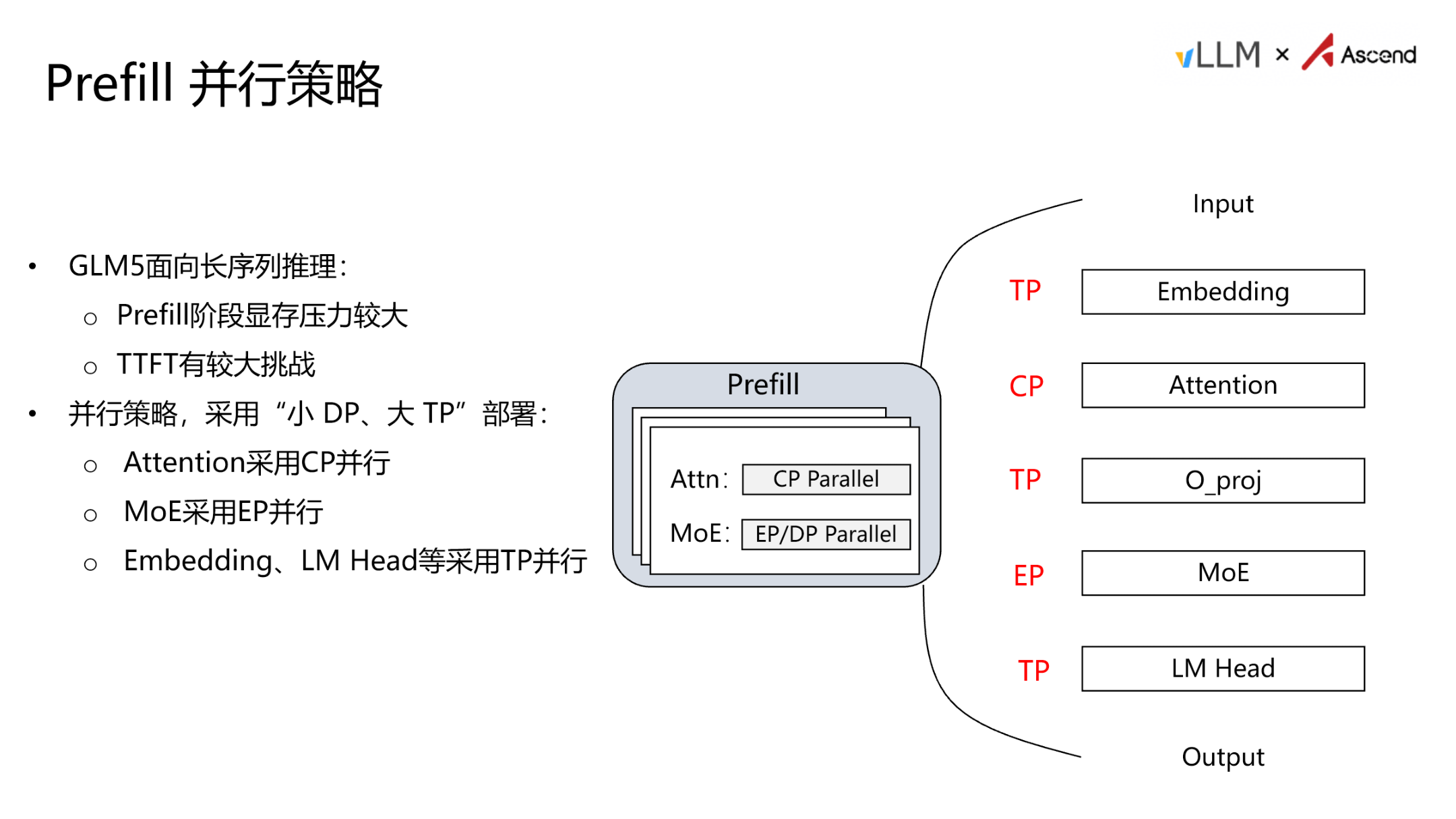Figure: Prefill parallelism strategy—Input flows through Embedding (TP), Attention (CP), O_proj (TP), MoE (EP), and LM Head (TP) to produce output. Source: PPT page 10

Key elements in the diagram:

• Embedding / LM Head → TP: Matrix multiplications are partitioned across cards via tensor parallelism—the most conventional parallelism approach.
• Attention → CP (Context Parallelism): This is the core technique for handling long sequences. CP partitions the input token sequence along the position dimension so that each card processes only a portion of the context. The benefits are twofold: the amount of KV Cache each card needs to store decreases linearly with the partition count, directly alleviating the memory bottleneck; CP's communication and computation can overlap, partially masking communication overhead.
• MoE → EP: Different experts are assigned to different devices, with tokens routed via All-to-All communication, so expert weights need not be stored in their entirety on every card.

The causal logic of this combination: long sequence → insufficient memory → use CP to partition the sequence + EP to partition experts → per-card load becomes manageable → TTFT target met.

Decode Stage: Large DP, Small TP

The D node's KV Cache is transferred on demand from P nodes, so its own memory pressure is lower. The bottleneck shifts to communication share—the larger the TP degree, the more cross-card communication is required per step, yet the effective data volume per communication is very small; an excessive communication share directly slows TPOT. Therefore, D nodes adopt a "large DP, small TP" strategy.

The following diagram illustrates the parallelism assignment for D nodes, forming a contrast with the P node strategy above:

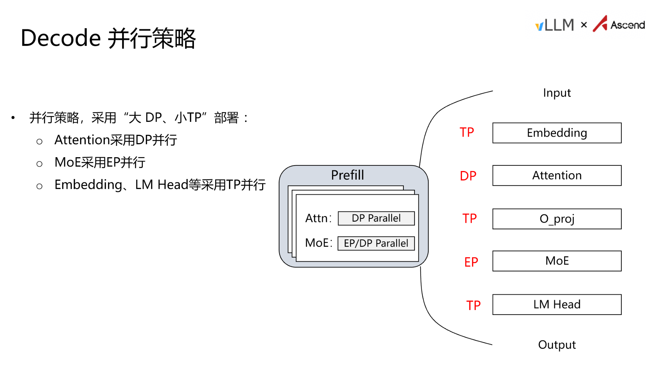Figure: Decode parallelism strategy—Attention is changed to DP parallelism; other modules remain the same. Source: PPT page 11 (the left-side box title in the original figure is mislabeled as "Prefill"; it actually describes the Decode strategy)

Compared to Prefill, the key change is concentrated in the Attention module: it is switched to DP, allowing each card to independently process different requests. Since the sequence length per Decode step is only 1, CP partitioning no longer serves any purpose.

Summary of strategy differences between the two stages:

Module	Prefill (P Node)	Decode (D Node)
Embedding / LM Head	TP	TP
Attention	CP	DP
MoE	EP	EP
DP degree	Small	Large
TP degree	Large	Small

Conclusion: PD disaggregation provides architecture-level assurance for long-sequence inference and is the prerequisite for achieving both low TTFT and low TPOT. An important boundary condition to note: PD disaggregation introduces the cross-node communication overhead of transferring KV Cache from P nodes to D nodes. For extremely long sequences, this transfer volume can be substantial; whether it becomes a new bottleneck depends on the inter-node interconnect bandwidth and the degree of KV Cache compression—the latter being exactly the topic of the next section.

---

5. Breaking the Memory Wall: Quantization Strategies and C8 KV Cache

Central question of this section: Without adding hardware, how can memory footprint be further compressed to increase the system's maximum concurrency?

Architectural decomposition addresses compute resource allocation, but the physical memory ceiling of individual nodes remains. When the combined footprint of model weights and KV Cache approaches the HBM boundary, the number of concurrent requests a single card can accommodate is still limited. The answer points to quantization along two dimensions—weight-activation quantization and KV Cache quantization.

Weight and Activation Quantization: W8A8 / W4A8

Quantization represents weights (W) and activations (A)—originally stored in BF16 (16-bit Brain Floating Point)—using lower-bitwidth integers, reducing the number of bytes per parameter. GLM-5 supports two quantization schemes on Ascend NPUs. The following table compares model weight memory footprint across three precision levels (data source: PPT page 12):

Precision Scheme	Weight Bitwidth	Activation Bitwidth	Weight Memory Footprint
BF16 (original)	16 bit	16 bit	1,510 GB
W8A8	8 bit	8 bit	764 GB
W4A8	4 bit	8 bit	395 GB

The above figures represent the total weight size of the entire model, excluding KV Cache and intermediate activations.

From BF16 to W8A8, weight footprint is reduced to approximately half; W4A8 is only 26% of the original. Deploying at full BF16 precision while maintaining stable operation in long-sequence scenarios requires far more resources than quantized schemes.

GLM-5 does not apply uniform precision to all submodules; instead, it differentiates based on each component's sensitivity to precision. In the configuration shown on PPT page 12, the SFA (Sparse Flash Attention) component of attention computation retains BF16, the Lightning Indexer uses A8C8 (8-bit activations, int8 cache), and the remaining linear projections and MoE expert layers use W8A8. Attention scores are more sensitive to numerical error, which is why SFA retains high precision.

C8 KV Cache: Returning Saved Memory to Concurrency

Weight quantization only addresses "static" footprint. In inference services, the KV Cache is the dynamic memory hog—it grows proportionally with sequence length × number of concurrent requests.

C8 KV Cache technology compresses the KV Cache from the default BF16/FP16 to int8 (8-bit integer) format for storage, directly halving the bytes per cache element. The causal chain is as follows:

KV Cache stored in int8
    → Per-token cache footprint reduced by approximately 50%
    → The same HBM capacity can hold cache for more tokens
    → The system can serve more concurrent requests simultaneously (or support longer contexts)
    → Overall throughput improves

Minimal numerical example: Suppose a single request's KV Cache occupies 200 MB under BF16; after int8 compression, it is approximately 100 MB. A card with 16 GB of free memory can accommodate at most 80 concurrent requests under BF16, but approximately 160 under C8 mode—the concurrency ceiling is directly doubled. (This example is a simplified calculation for illustrative purposes; actual values depend on sequence length, number of layers, and attention head dimensions.)

Precision Boundaries and Hardware Compatibility

On current Ascend 910B / 910C hardware, C8 refers exclusively to int8. Future iterations of the 910 series will support FP8 format, at which point the scope of C8 will also expand. The costs of quantization include:

1. Precision loss—Output quality may degrade in certain scenarios; this must be evaluated against business tolerance.
2. Operator adaptation—In the W4A8 scenario, weights are stored at 4 bits but computed at 8 bits, involving a dequantization process. Currently, fused operators merge dequantization with matrix multiplication to avoid the extra latency of a standalone call.
3. Not all submodules are suitable for low precision—SFA still maintains BF16, demonstrating that quantization strategies must be evaluated on a per-module basis.

Conclusion: Quantization is the most direct means of increasing concurrency under a fixed hardware budget. Weight quantization compresses static footprint, C8 KV Cache compresses dynamic footprint, and the combination can significantly increase the deployable scale of the system. However, per-module precision assignment and the hardware's support range for low-precision formats determine the practical ceiling of the quantization strategy.

---

6. Low-Level Acceleration: Graph Mode and Custom Fused Operators

Central question of this section: How can operator dispatch latency be reduced and execution efficiency of complex structures like MoE be improved?

Once the memory capacity issue is mitigated, the system's performance bottleneck may shift to the framework layer: the cumulative latency of dispatching each operator from CPU to NPU can exceed the operators' actual execution time on the accelerator. Moreover, MoE generates substantial intermediate data movement across the dispatch, compute, and combine phases. This section dissects two low-level techniques: graph mode to eliminate scheduling overhead, and fused operators to eliminate redundant data movement and communication stalls.

ACL Graph: Capture Once, Replay Repeatedly

ACL Graph is the graph mode technology on the Ascend platform, analogous to NVIDIA's CUDA Graph. Its workflow can be summarized in three steps:

Phase	Behavior	Benefit
Capture	During the first execution, the framework records a sequence of operators' shapes, parameters, and dependencies as a static computation graph	Occurs only once
Compile	Performs offline optimizations on the graph such as operator fusion and memory planning	Generates an efficient dispatch instruction sequence
Replay	In all subsequent inference calls, the entire graph is submitted to the NPU in a single dispatch	Transforms "per-operator dispatch" into "whole-graph single dispatch"

Why is this especially critical for Decode? In the Decode stage, each step generates only one token; per-operator computation is extremely small, and the CPU-side per-operator dispatch latency can far exceed the operator execution itself. After enabling ACL Graph, improvements are observable in both TTFT and TPOT.

Boundary condition: Graph mode requires operator shapes to remain unchanged after capture; for dynamic-shape scenarios (e.g., variable-length sequences), shape bucketing is typically needed to maintain static graph reuse rates.

Fused Operators: Two Key Cases

GLM-5 implements multiple custom fused operators on Ascend, the most representative of which are MLAProlog and DispatchFFNCombine. The following diagram illustrates the internal structure and execution timeline of these two fused operators—a key reference for understanding the low-level acceleration principles:

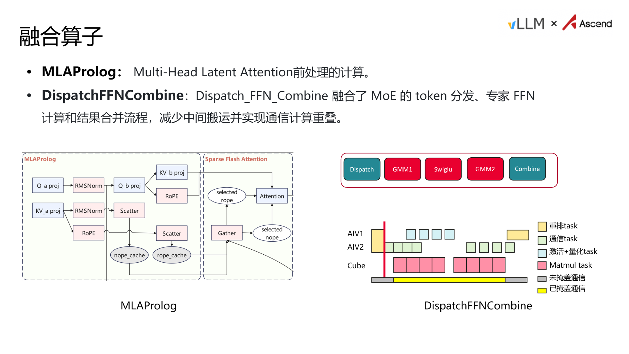Figure: Left—MLAProlog data flow; Right—DispatchFFNCombine Gantt chart timeline. Source: PPT page 14

MLAProlog—Attention Preprocessing in a Single Step

Multi-Head Latent Attention (MLA) requires a series of preprocessing operations before entering the attention computation, including Q/KV projections (Q_a_proj, KV_a_proj, etc.) and RoPE positional encoding. Without fusion, these operations are dispatched as independent operators sequentially, each incurring a CPU→NPU scheduling overhead and an intermediate tensor read/write to HBM.

MLAProlog fuses all preprocessing computations into a single operator kernel, completing everything from projection to encoding in one invocation. The benefits are twofold: scheduling overhead drops from N times to once; intermediate tensors no longer write back to HBM but flow directly to the next step in on-chip SRAM.

DispatchFFNCombine—MoE Communication-Compute Fusion

The standard execution flow of an MoE layer is Dispatch → GMM1 → SwiGLU → GMM2 → Combine. Dispatch routes each token to its corresponding expert; Combine merges expert outputs by weight. If executed serially, Dispatch and Combine involve cross-card communication, during which the compute units sit idle waiting for communication to complete.

The Gantt chart on the right side of the diagram above clearly shows the before-and-after comparison. After optimization, execution is decomposed across different hardware units for parallel processing via task-level rescheduling:

Hardware Unit	Task Type Handled
AIV1	Reorder tasks, activation + quantization tasks
AIV2	Communication tasks
Cube	Matmul tasks

The key insight: while AIV2 executes communication tasks, the Cube can simultaneously execute matmul tasks—the "masked communication" region in the diagram. In the ideal case, communication latency is completely hidden by computation; in practice, a small portion remains that cannot be overlapped, but overall MoE layer execution efficiency improves significantly.

MTP: Trading Extra Compute for Multi-Token Output

MTP (Multi-Token Prediction) adds an extra computation layer on top of the standard structure, enabling each Decode round to output multiple candidate tokens.

However, MTP is not a case of "bigger is better." The acceptance rate decreases as the MTP value increases: when MTP is set too high, most of the additionally predicted tokens are discarded, while the latency overhead from the extra computation layer is fixed—resulting in a negative net benefit. The appropriate MTP value should be selected based on the actual token distribution of the business workload.

Conclusion: Graph mode and fused operators compress ineffective framework overhead along two dimensions—the scheduling path and the execution path, respectively. ACL Graph transforms per-operator dispatch into whole-graph replay; MLAProlog and DispatchFFNCombine eliminate intermediate data movement and achieve communication-compute overlap through hardware-unit-level task parallelism. These low-level techniques are essential for breaking through the framework's performance ceiling and unlocking the hardware's computational potential.

---

7. End-to-End Performance Validation and Extreme Scenario Analysis

Central question of this section: After combining all the optimization techniques described above, how does GLM-5 perform in real high-concurrency scenarios? Which test conditions have a decisive impact on results?

After full-stack optimization from architecture to operator level, the combined end-to-end benefits must ultimately be validated in complex business scenarios. The following data are from a PD-disaggregated deployment configuration (PPT page 15):

Multi-Scenario Performance Panorama

Avg Input	Avg Output	Prefix Cache Hit Rate	Parallelism Strategy (P / D)	Max Concurrency	Request Rate (req/s)	TTFT Mean (ms)	TPOT Mean (ms)	TPS
16K	1K	0%	DP4 TP8 / DP8 TP4	112	1.5	30,825	22.5	1,205
64K	1K	90%	DP2 TP16 / DP8 TP4	256	0	64,367	34.1	2,354
128K	1K	90%	DP2 TP16 / DP8 TP4	120	1	28,334	25.2	934
64K	256	90%	DP2 TP16 / DP32 TP2	200	4.2	8,009	21.2	932
64K	1K	90%	DP2 TP16 / DP32 TP2	200	4	7,738	32.8	3,059

Prefix Cache hit rate refers to the proportion of input prefixes that can be reused across requests; the higher the hit rate, the fewer tokens the Prefill stage actually needs to recompute.

Row-by-Row Analysis of Key Variables

Highest throughput row (Row 5). Under conditions of 64K input, 1K output, and 90% Prefix Cache hit rate, the Decode side is expanded to DP32 TP2—32-way data parallelism with only 2 cards of tensor parallelism per replica. The request rate is controlled at 4 req/s, TTFT drops to approximately 7.7 s, and TPS reaches 3,059. This is the peak throughput across all scenarios in the table.

Extreme TTFT row (Row 2). Also 64K + 90% cache hit, but the request rate is marked as 0—all 256 requests flood the Prefill node at the same instant. TTFT surges to 64,367 ms (approximately 64 seconds), nearly an order of magnitude higher than Row 5, while TPS is 2,354—not the highest.

128K long-context row (Row 3). When the input doubles to 128K, even with a request rate reduced to 1 req/s, TTFT remains in the 28-second range. The impact of sequence length on Prefill computation is close to quadratic—it is the most direct amplification factor for TTFT.

Short output row (Row 4). When output length is shortened from 1K to 256 tokens, TPS drops from 3,059 to 932. TPS measures output tokens per second; when each request generates fewer tokens, total output token volume decreases even if processing speed is similar. TPOT, conversely, is the lowest in the entire table (21.2 ms), indicating that Decode itself is not the bottleneck.

Causal Chain of Instantaneous Concurrency

The 64-second TTFT in Row 2 is not a system malfunction but a reproducible boundary behavior:

1. Request rate is 0 → All 256 64K requests arrive at the Prefill node at the same instant.
2. The P node uses DP2 TP16, providing only 2 data-parallel instances; each instance must queue approximately 128 64K-length sequences.
3. A single 64K Prefill itself takes on the order of seconds; after queuing 128, the cumulative wait time for the last completed request reaches approximately 64 seconds.
4. The Decode node uses only DP8 TP4 (rather than Row 5's DP32 TP2), so generation-stage parallelism is relatively low.

In contrast, Row 5: requests arrive at a steady rate of 4 req/s, keeping the Prefill node's queue depth consistently manageable, reducing TTFT to 7.7 s; upgrading the Decode side to DP32 TP2 further unlocks throughput, with TPS leaping to 3,059.

State Comparison Under Identical Configuration but Different Traffic Patterns

With 64K input, 1K output, and 90% cache hit rate held constant:

Comparison Dimension	Instantaneous Burst (Row 2)	Steady-State Arrival (Row 5)
Request rate	0 (all at once)	4 req/s
Decode parallelism strategy	DP8 TP4	DP32 TP2
TTFT	64,367 ms	7,738 ms
TPOT	34.1 ms	32.8 ms
TPS	2,354	3,059

TPOT is virtually unaffected by the traffic pattern (difference < 4%), because the per-token generation speed of an individual request within Decode is determined by hardware and model structure. In contrast, TTFT and TPS are highly sensitive to the request arrival pattern and Decode-side parallelism degree.

Conclusions and Boundary Conditions

By combining PD disaggregation, Prefix Cache, and a large-DP/small-TP Decode parallelism strategy, GLM-5 achieves an output throughput of 3,059 TPS in 64K long-context scenarios on the Ascend platform. However, this number rests on a set of prerequisites, none of which can be omitted:

• 90% Prefix Cache hit rate—whether this is achievable in practice depends on the degree of prefix overlap among requests;
• Steady-state request arrivals—instantaneous concurrency causes Prefill queue buildup, degrading TTFT to the minute-level;
• Sufficient Decode-side scaling—DP32 TP2 requires 64 cards; the resource cost is not negligible.

---

Summary

This article follows the causal chain of "metric definition → bottleneck identification → architectural decomposition → data compression → operator acceleration → end-to-end validation" to systematically dissect the inference optimization path of GLM-5 on the Ascend platform. The core conclusions are as follows:

1. Inference optimization is a systems engineering effort that requires finding the optimal equilibrium—grounded in business SLOs—among latency (TTFT/TPOT), throughput (TPS), and memory. The four-step analytical framework (define metrics → identify bottlenecks → select strategies → validate quantitatively) is the prerequisite for all optimization decisions.

2. GLM-5's Lightning Indexer constitutes a significant bottleneck under long sequences. The module's TopK computation accounts for 26.53% of Prefill stage latency in long-context scenarios, making it the single largest hotspot in the entire inference pipeline.

3. PD disaggregation architecture effectively decouples compute-bound and memory-bound tasks. Prefill uses "small DP, large TP + CP" to distribute compute and memory pressure; Decode uses "large DP, small TP" to reduce communication share and boost concurrency.

4. Quantization is the most direct means of expanding concurrency capacity. W4A8 compresses weight memory from 1,510 GB to 395 GB; C8 KV Cache halves dynamic cache footprint; the combination significantly increases the deployable scale.

5. Hardware–software co-optimized low-level acceleration is indispensable. ACL Graph eliminates operator dispatch overhead; the MLAProlog and DispatchFFNCombine fused operators eliminate intermediate data movement and achieve communication-compute overlap—these are the keys to breaking through the framework-layer performance ceiling.

6. End-to-end performance is highly sensitive to test conditions. The peak throughput of 3,059 TPS holds under the specific premises of 64K input, 1K output, 90% Prefix Cache hit rate, 4 req/s steady-state arrival, and P: DP2 TP16 / D: DP32 TP2; instantaneous concurrency can degrade TTFT to 64 seconds.

Stated limitations:

• All performance data in this article come from publicly presented test results in the speaker's PPT slides and do not include quantitative evaluations of different Prefix Cache hit rate gradients, higher DP configurations on the Prefill node, or the impact of quantization precision loss on output quality.
• The growth trend of TopK latency under long sequences was described verbally by the presenter; the precise complexity curve was not provided in the materials.
• The cross-node KV Cache transfer overhead introduced by PD disaggregation was not accompanied by published bandwidth data or latency impact figures in the materials.
• The precision impact of per-module quantization configurations (e.g., SFA retaining BF16, Lightning Indexer using A8C8) requires independent validation in specific business scenarios.