Core Analysis of vLLM-Omni: Asynchronous Batch Processing for Diffusion and the PiD Architecture in Practice

Source video: Bilibili BV189816ZE9C · Slides: BilibiliShare deck

Online inference for diffusion models presents a hard-to-reconcile contradiction: at small resolutions the GPU compute capacity is underutilized, while at large resolutions memory consumption and latency remain stubbornly high. vLLM-Omni addresses this by first decomposing the scheduling granularity from "entire request" down to "single denoising step," enabling dynamic batching between steps to boost throughput on small shapes; and then introducing PiD (Pixel Diffusion) to replace VAE decode, so that the main model always performs inference at a small resolution while a lightweight super-resolution module upscales to the target size. This article follows that causal chain, starting from the blocking problem and progressively dissecting asynchronous scheduling, dynamic batching, heterogeneous-resolution handling, performance boundaries, and the mechanism and measured benefits of PiD.

Target audience: AI engineers and backend developers with a foundation in deep-learning inference who are interested in model deployment and performance optimization.

Prerequisites: Familiarity with basic concepts of the diffusion-model denoising process (steps, latents, noise schedules), general principles of batched inference, and an introductory understanding of the attention mechanism.

Reading objectives:

1. Understand the root cause of compute underutilization in traditional synchronous diffusion inference.
2. Master vLLM-Omni's step-granularity asynchronous request dispatch and dynamic batching mechanism.
3. Learn the chunking and attention-isolation strategies for batching requests with heterogeneous resolutions.
4. Recognize how PiD combines early termination with upsampling to achieve both high throughput at small resolutions and high-resolution image generation.

---

1 The Engineering Contradiction of Synchronous Scheduling: Why Does Diffusion Need to Go Asynchronous?

Core question of this section: Why does the traditional diffusion inference interface cause GPU compute to sit idle?

Why Request-Granularity Synchronous Execution Becomes a Bottleneck

In vLLM-Omni's multi-stage pipeline, generation requests enter the Diffusion stage after the upstream AR (autoregressive) stage completes. Before the redesign, the Diffusion Engine dispatched tasks to backend Workers synchronously at the request granularity—meaning a single request had to run through all denoising steps (each step being one noise-removal computation in the diffusion generation process) before releasing the execution channel, forcing subsequent requests to queue.

This means that even if the GPU has parallel headroom while processing a single request, newly arriving requests cannot be incorporated into the current computation. The prerequisite for dynamic batching (combining multiple independent inference requests into a single batch for parallel computation to improve GPU utilization) is "gathering a set of compatible requests," but under the synchronous model this prerequisite can never be met.

How Blocking Devours Batching Opportunities

The figure below illustrates the motivation for the asynchronous redesign and the overall architecture. Focus on the Motivation area in the upper-left corner and the causal chain it describes:

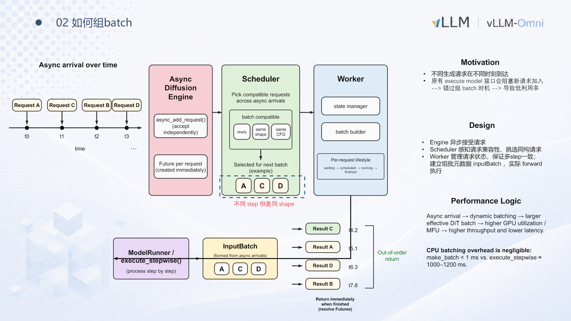Caption: The left side illustrates requests arriving asynchronously over time; the center shows the three-tier responsibilities of Engine → Scheduler → Worker; the right side explains that results are returned out of order as each request completes. Source: presentation slide 5.

The Motivation section in the figure lays out a three-part causal chain:

#	Stage	Explanation
①	Different generation requests arrive at different times	In real-world scenarios requests are naturally asynchronous with unpredictable inter-arrival intervals
②	The original execute model interface blocks new requests from joining	The execution granularity is all steps of an entire request, monopolizing the channel
③	Missed batching opportunities → low utilization	Concurrent requests cannot be merged into the same batch, wasting GPU parallelism

The "Out-of-order return" label on the right side of the figure hints at the redesign direction: if requests can complete and return independently, the constraint of "one request locking down the entire channel" is broken.

A Minimal Timeline: What Exactly Does Blocking Waste?

Assume four requests A–D arrive at t₀–t₃ respectively, each requiring multiple denoising steps. Under synchronous mode:

t₀ ──── A executes all steps ────── A completes
                                     t_done_A ── B executes all steps ── B completes
                                                                          ...

Request B has already arrived at t₁ but must wait until A finishes before it can start. Each request monopolizes the GPU, the batch size is always 1, and matrix compute units sit largely idle.

With batching enabled: once the Scheduler determines that A, B, and D share the same shape and CFG (Classifier-Free Guidance scale) configuration, they can be merged into a single batch for parallel execution, effectively increasing throughput.

Summary

The fundamental problem with synchronous execution is a mismatch between execution granularity and scheduling granularity: scheduling operates at the "entire request" level, yet diffusion generation is inherently composed of multiple steps with natural scheduling windows between them. Decomposing the granularity from request-level to step-level opens the door to dynamic batching. This is precisely the core design explored in the next section.

---

2 Core Design: Step-Granularity Asynchronous Request Dispatch

Core question of this section: How can the scheduling granularity be broken down from request-level to step-level, so the system can insert, terminate, or return requests between any two steps?

The Pre-Redesign Bottleneck

Before the redesign, the upper stage (the request-parsing and dispatch layer spun up by the FastAPI service) handed requests to the Diffusion stage synchronously. The entire chain was serially blocked:

Aspect	Pre-redesign behavior	Direct consequence
Dispatch granularity	Synchronous wait per request	The engine holds only one request at a time
Batching	Impossible	Low GPU utilization
Interrupt responsiveness	Must wait for all steps to complete before returning	Cannot terminate long-running requests early

Overall Interaction Flow

The figure below is a sequence diagram of asynchronous dispatch, showing the message flow among four actors: the client thread, DiffusionEngine, StepScheduler, and the Worker:

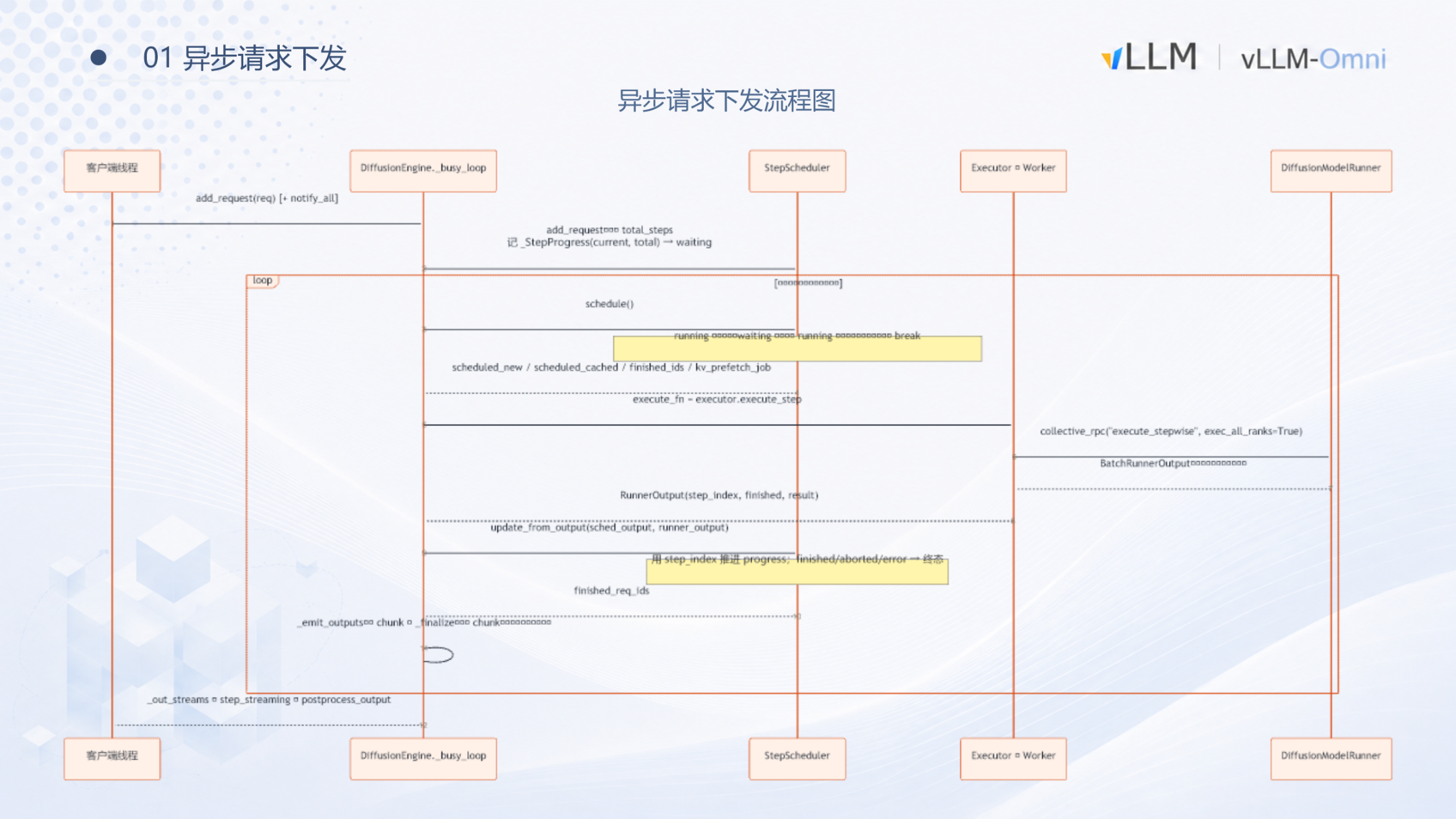Caption: Asynchronous request dispatch sequence diagram, showing the complete path from request enqueuing, scheduling, per-step execution, to streaming result return. Source: presentation slide 3.

The four lifelines from left to right correspond to: the upper-stage client thread (producer), DiffusionEngine._busy_loop (scheduling heartbeat), StepScheduler (queue management), and Executor/Worker + DiffusionModelRunner (consumer). The message arrows form a closed loop of "enqueue → loop-schedule → step-execute → stream-return."

The Three-Part Causal Chain

① Producer: Enqueue and Return Immediately

When an upper-stage thread receives a Diffusion request, it performs two actions and then relinquishes its responsibility:

1. Calls _add_prepared_request to place the request into the StepScheduler's waiting queue and wakes the background loop;
2. Calls get_output_stream to obtain an asynchronous output stream handle for receiving results later.

The fundamental difference from the pre-redesign approach is that the producer is only responsible for "insertion" and "stream subscription"—it no longer blocks waiting for the entire request to finish all denoising steps. When the first request arrives, _check_and_start_background_loop is additionally triggered to initialize the thread locks and asyncio variables required for queue read/write operations.

② Scheduling Hub: _busy_loop

DiffusionEngine maintains an internal background thread called _busy_loop, which serves as the heartbeat of the entire asynchronous mechanism. Its behavior can be simplified to an infinite loop:

1. Read currently schedulable requests from StepScheduler (schedule / deschedule);
2. If schedulable requests exist, package them and send them to the backend Worker to execute one step;
3. After the step completes, write intermediate results or final outputs back to each request's corresponding output stream;
4. Return to step 1 and begin the next iteration.

If no schedulable requests are available, the thread suspends via a wait/notify mechanism to avoid busy-waiting on CPU, and is explicitly notified when a new request is enqueued.

StepScheduler itself maintains two queue categories: running and waiting. In each loop iteration, the scheduler checks which requests in the waiting queue have met their execution conditions, promotes them to the running queue, and together with the existing running requests forms the batch for the current step.

③ Consumer: Per-Step Execution and Return

When the Worker receives a batch of requests, it concatenates each request's latent (the intermediate data representation processed during the diffusion denoising procedure, residing in latent space) along the tensor dimension and hands the result to DiffusionModelRunner for one denoising computation. After computation, results are split by request and streamed back to their respective client threads via the output streams.

After each step completes, control returns to _busy_loop. This opens a window for three operations:

• Insert new requests: Newly arrived requests are pulled into the running queue in the next loop iteration and immediately participate in batching.
• Terminate requests: After the upper layer issues an interrupt signal, _busy_loop removes the target request in the next iteration.
• Return intermediate results: Requests that have completed all steps output the final image; requests still in progress can output the current step's intermediate latent.

Minimal State-Evolution Example

Assume the system starts empty and requests A and B arrive successively:

Time	Event	StepScheduler state	Worker execution
t₀	A enqueued, busy_loop woken	waiting→running:	—
t₁	A's step 1 completes	running:	A step 1
t₂	B enqueued (in the inter-step gap)	waiting→running:	—
t₃	A step 2 + B step 1 batched together	running:	{A, B} batch execution
t₄	A finishes all steps, result output	running:	B continues step 2…

B does not need to wait for A to finish all denoising steps before joining. It is pulled into the running queue by the scheduler during the inter-step gap at t₂ and shares the same GPU computation with A starting from t₃.

Boundary Conditions

1. The smaller the model and the faster each step, the higher the scheduling overhead ratio. When the GPU computation for a single step is itself very short, millisecond-level scheduling overhead becomes non-negligible.
2. Interrupt response granularity is "before the next step begins." If a single step takes a long time, the actual interrupt latency equals the remaining execution time of the current step.
3. The presentation materials did not disclose the specific priority rules inside StepScheduler or the maximum number of requests per batch.

Summary: Pushing the scheduling granularity down from request to step is the foundational infrastructure for all subsequent batching optimizations. It gives DiffusionEngine the ability to dynamically add or remove requests in the gap between every denoising step, while natively supporting interrupts and streaming of intermediate results. With this flexibility in place, the immediate follow-up question is: does the CPU overhead of assembling a batch within the extremely short inter-step gap become the new bottleneck?

---

3 Data Structures and Execution: Ultra-Low-Overhead Dynamic Batching

Core question of this section: Between every two steps, the CPU side must complete request filtering, padding computation, and mask construction—do these operations become a new performance bottleneck?

The answer is no. According to the profiling data presented in the talk, the core batching function make_batch takes < 1 ms, while the GPU-side execute_stepwise for a single denoising step takes roughly 1,000–1,200 ms. The two differ by three orders of magnitude; the CPU scheduling overhead is entirely hidden behind GPU computation time.

Why Requests at Different Progress Points Can Share the Same Batch

The prerequisite for batching is that merging must not alter the computational semantics of any individual request. A diffusion model has three dimensions that may differ across requests:

Dimension	Does it affect the forward pass?	Handling strategy
Denoising progress (timestep)	No—timestep is a per-request conditional input	Each request independently tracks its current step
Text length (number of text tokens)	Affects tensor width	Pad to the current batch-internal maximum length \(T_{\max}\), with an attention mask
Image size (latent resolution)	Affects tensor height	The current scheme requires matching shapes for merging

Together, these three rules form the compatibility criteria the scheduler uses when selecting requests: only requests with the same shape and the same CFG configuration are selected into the same batch.

Key Data Structures: RequestState and InputBatch

The figure below shows how two core structures collaborate to go from per-request state management to unified tensor construction:

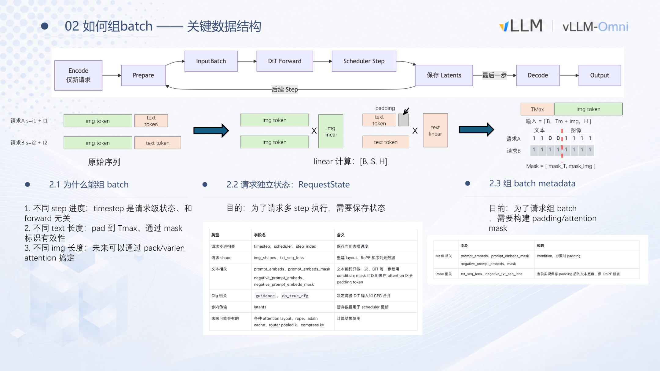Caption: Batching data structures and tensor construction flow. Source: presentation slide 6.

RequestState—Per-Request State Container

Every generation request entering the system corresponds to a RequestState instance that stores at least the following information:

• Current timestep: The number of completed denoising steps, determining which timestep embedding to use for the next step.
• Latent tensor: The intermediate denoising result at the current step, with shape corresponding to the target image resolution.
• Text embedding: The conditional vector produced by the text encoder; remains constant across multiple steps to avoid redundant encoding.
• CFG parameters: Configuration such as the Classifier-Free Guidance scale.

RequestState fully decouples the request lifecycle (waiting → scheduled → running → finished) from GPU single-step execution. The scheduler only needs to read each request's state fields to determine which requests are eligible for merging.

InputBatch—Batch Metadata and Unified Tensors

After the scheduler selects a group of compatible requests, the batch builder in the Worker assembles them into an InputBatch in three steps:

1. Text padding: Suppose request A has text length \(s_A\) and request B has \(s_B\); let \(T_{\max} = \max(s_A, s_B)\). The shorter sequence is zero-padded at the tail so that all text tensors align to \([B,\; T_{\max},\; H]\).
2. Mask construction: Two sets of masks are generated—mask_T (valid text positions) and mask_Img (valid image-token positions)—so that invalid positions are masked out during attention computation.
3. Tensor concatenation: The text portion and the image latent portion are concatenated along the sequence dimension, yielding a final input shape of \([B,\; T_{\max} + L_{\text{img}},\; H]\).

Once assembly is complete, the GPU needs only a single DiT (Diffusion Transformer) forward pass to advance all requests in the batch by one step.

Minimal State-Evolution Example

Request	Target resolution	Text length	Current step	CFG
A	512×512	48	3	7.5
B	512×512	32	1	7.5
C	1024×1024	60	0	7.5

Scheduler decision: A and B share the same resolution and CFG, so they can be merged; C has a different resolution and must be executed separately or wait for a same-resolution request.

InputBatch construction (A + B): \(T_{\max} = 48\); B's text is padded with 16 zero vectors; latent shapes are identical, requiring no additional processing; the timestep vector is \([t_A^{(3)},\; t_B^{(1)}]\), each corresponding to the noise schedule value of its respective denoising stage.

After one GPU step, A advances to step 4 and B to step 2. If A's total step count is 4, A is marked as finished and its Future resolves immediately, returning the result—the return order is independent of the arrival order.

Boundary Conditions and Current Limitations

1. Same-shape constraint: Requests with different resolutions cannot be merged. In real-world workloads users often request varying target sizes, which significantly limits the effective batch size.
2. CFG consistency requirement: Requests with different guidance scales also cannot be merged, further shrinking the pool of batchable requests.

Summary: The CPU scheduling overhead of batching is negligible in the current implementation. The real factor constraining dynamic batching effectiveness is shape and configuration heterogeneity across requests. When requests with multiple resolutions coexist, can they be placed into the same batch?

---

4 Batching Strategy for Heterogeneous Resolutions

Core question of this section: When concurrently arriving requests have different resolutions—e.g., 1024×1024, 768×768, and 512×1024—and tensor shapes cannot be aligned, can they still be placed into the same batch for parallel execution?

From Homogeneous to Heterogeneous: A New Engineering Contradiction

In the homogeneous case all latents share the same spatial dimensions and can be directly concatenated along the batch dimension. Once resolutions differ, the core contradiction becomes: latent tensors have unequal lengths in the spatial dimension and cannot form a regular [B, S, H] tensor. Naïve padding alignment wastes massive compute and memory, while serial execution leads to low GPU utilization.

Equal-Length Chunk Splitting and Reassembly

The key idea: rather than concatenating at the original resolution, first split each request's image latent into equal-length chunks, then batch all chunks together for execution.

1. Compute the splitting granularity—Take the greatest common divisor (GCD) of the image heights and widths across all requests to determine the chunk spatial size. For example, given three requests with resolutions 1024×1024, 768×768, and 512×1024, the GCD yields 256×256 chunks.
2. Split—Each request's latent is divided by chunk size. A 1024×1024 latent produces 16 chunks; a 768×768 latent produces 9.
3. Concatenate—All chunks are treated as independent "small image" token sequences and concatenated along the batch dimension into one large tensor, then fed uniformly into the DiT block.
4. Reassemble—After denoising, chunks belonging to the same request are reassembled at their original positions to recover the complete image.

Why Only Self-Attention Requires Special Treatment

Operators inside a DiT block can be classified by whether they require cross-chunk context:

• No cross-chunk dependency: Linear layers, LayerNorm / RMSNorm, element-wise operations—they operate independently on each token, so splitting does not affect the result.
• Cross-chunk dependency: Self-attention is the sole exception. Its Q, K, V interactions span all spatial positions within the same image; performing attention only within a chunk is equivalent to imposing a local window, which causes accuracy loss.

Therefore, after batching only the self-attention step requires special treatment; all other operators execute directly at chunk-granularity in the large batch.

Two Approaches for Self-Attention

Approach 1: Recover before attention, scatter after attention (Recover-Scatter). Before entering self-attention, all chunks belonging to the same request are reassembled to the original resolution shape; requests sharing the same resolution can be grouped into a small batch for joint computation; after completion, the result is split back into chunk form to continue through subsequent layers.

Approach 2: Varlen Attention Mask. Varlen attention (Variable-Length Attention) allows specifying precisely which K/V tokens each Q token should interact with via a variance mask, eliminating the need for physical recover/scatter operations and reducing data movement overhead. The speaker noted that this functionality was not yet available during their early work and represents a newer optimization path.

Where the Gains Come From

The batching gains come primarily from all operators other than attention. Linear, Norm, and element-wise operations form larger batches at chunk granularity, allowing GPU compute units to be utilized more fully. The attention stage maintains accuracy through the two approaches described above—it introduces no additional gains but also no losses.

Boundary Conditions

• When the GCD is very small: Extreme resolution differences cause the chunk count to explode and the attention recovery overhead to grow, potentially negating the gains.
• VAE decode remains serial: VAE decode is a memory-bound operation with limited batching gains; it is currently executed serially.

Summary: Through GCD-driven equal-length chunk splitting, requests with heterogeneous resolutions can share batch execution across all operators except self-attention, improving GPU utilization with no accuracy loss. With the mechanism design complete, the next step is to verify the real-world gains at different resolutions through measured data.

---

5 Performance and Bottlenecks: Where Are the Batching Gain Boundaries?

Core question of this section: After enabling batching, do throughput and latency improve significantly at all resolutions?

The answer is no. The magnitude of the gains depends on how saturated the GPU compute is when generating a single image: the larger the shape and the fuller the compute, the less headroom batching can unlock. All data below are based on measurements of the Qwen-Image model on a single Ascend A3 card.

1024×1024: Compute Already Saturated, Near-Zero Gains

At 1024×1024 resolution, throughput without batching holds at approximately 0.0127 req/s. With batching enabled it edges up to 0.0131 req/s—a lift of less than 4%, essentially within measurement error.

Metric	Without batching	With batching	Change
Throughput (req/s)	≈ 0.0127	≈ 0.0131	≈ +3%
Latency growth trend	Linear	Approximately linear (slightly lower slope)	Minimal

The reason is intuitive: at 1024×1024 the matrix computation per step is sufficient to "saturate" the compute units; the bottleneck is compute capacity itself (compute bound) rather than scheduling gaps.

512×512: Small Shapes Unlock Significant Dividends

When the resolution drops to 512×512, the situation changes qualitatively. At Batch Size = 8:

Metric	Without batching	With batching (BS=8)	Change
Throughput (req/s)	≈ 0.1115	≈ 0.20	≈ +45%
E2E latency (s)	72	38	−33 s

At small shapes the per-image per-step computation is insufficient to fill the hardware, leaving large numbers of idle cycles. Batching concatenates the latents of multiple requests and sends them through in a single pass, filling exactly those idle cycles.

Gain Decomposition: Where Do 11 of Those 33 Seconds Come From?

By profiling the top-3 time-consuming operators (aclnnAddmm, aclnnMul, aclnnFA), the gains can be decomposed into two components:

1. Amortization of operator dispatch overhead: Without batching, each image's every step requires the CPU to independently dispatch a full suite of operator calls to the accelerator. With batching, multiple requests share the same dispatch round, keeping the call count on par with a single request. This alone saves 11 seconds, accounting for 34% of the total gain.
2. Improved compute utilization: The remaining ~22 seconds (66%) come from fuller utilization of hardware compute units.

The figure below contains three sub-charts corresponding to latency & throughput, operator dispatch time, and NPU utilization:

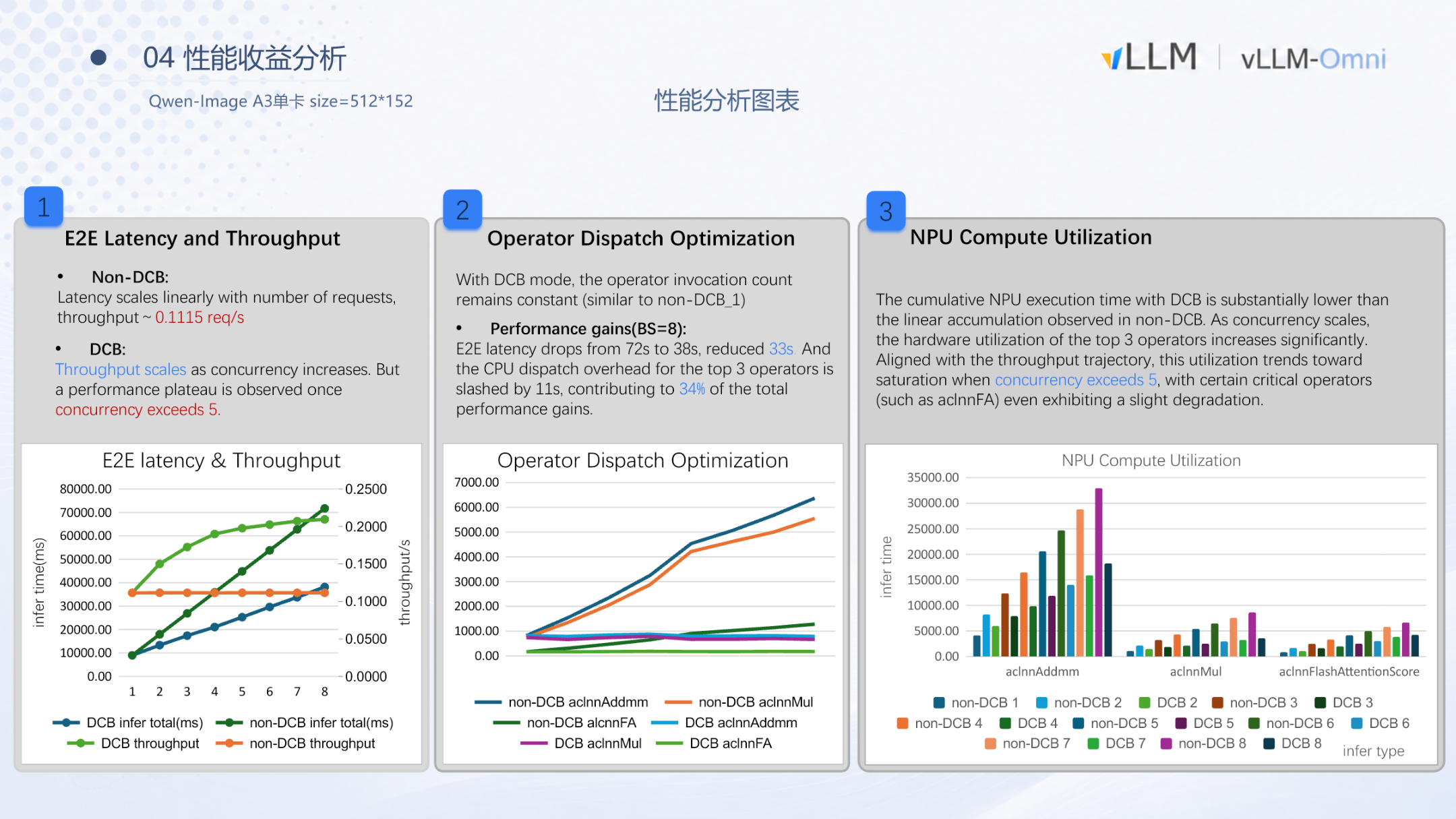Caption: Left chart shows E2E latency and throughput with and without batching at different concurrency levels; center chart shows how top-3 operator dispatch times change with concurrency; right chart shows NPU compute utilization as a bar graph. Source: presentation slide 9.

Key signals in the figure:

• Left chart: Without batching the latency curve rises strictly linearly with flat throughput; with batching the latency slope is noticeably lower and the throughput curve steadily climbs.
• Center chart: Without batching, dispatch time scales linearly with concurrency; with batching it stays nearly flat—confirming that operator call counts do not increase with batch size.
• Right chart: aclnnAddmm and aclnnMul show significant utilization gains under batching as concurrency rises, but aclnnFA (the FlashAttention operator) exhibits a slight decline at high concurrency, hinting at an additional scheduling bottleneck for attention computation on this hardware.

The Plateau Beyond Concurrency > 5

For both the throughput curve and NPU utilization, growth flattens once concurrency exceeds 5. Hardware utilization approaches its ceiling; further increasing the batch size only adds memory consumption without yielding more throughput. In practice, setting the batch size to 5–8 is a reasonable operating point.

Summary

Condition	Batching gain	Bottleneck
Large shape (1024×1024)	Minimal (< 4%)	Compute bound; capacity already saturated
Small shape (512×512), concurrency ≤ 5	Significant (throughput +45%, latency −33 s)	Operator dispatch + idle compute
Small shape, concurrency > 5	Diminishing marginal returns, entering plateau	Hardware utilization approaching saturation

The gains from batching fundamentally come from "filling idle compute + amortizing dispatch overhead." When both sources of headroom are squeezed to their limits, gains hit a ceiling. The data above are based on single-card Ascend A3 tests; saturation points on different hardware platforms may differ.

This raises a practical contradiction: batching works exceptionally well at small resolutions, but users often need high-resolution images. Is there a way to perform efficient inference on small latent shapes and still output high-resolution images?

---

6 Mechanism Deep Dive: PiD Early Termination and Feature Upsampling

Core question of this section: Can the bulk of the denoising be performed on small latents and the result then be "scaled up" to high resolution?

PiD (Pixel Diffusion) is designed precisely for this purpose. It replaces the traditional VAE decode stage, allowing early termination during an intermediate denoising step and using small-resolution features to generate a high-resolution pixel image.

From the Standard Pipeline to Early Termination

A typical diffusion image-generation pipeline comprises three stages:

Stage	Operating space	Purpose
VAE encode	Pixels → latent	Maps input to a low-dimensional latent space
Multi-step denoising (step 0 … N−1)	Latent	DiT blocks progressively denoise
VAE decode	Latent → pixels	Reconstructs the final latent into a pixel image

PiD intervenes at the third stage: it replaces VAE decode and does not require denoising to run all N steps—it can terminate early at intermediate steps such as N−2 or N−4, handing the latent at that point to PiD. The number of main-model inference steps is correspondingly reduced, lowering the compute cost of the denoising phase.

PiD Internal Structure: Three Inputs, One High-Resolution Output

The figure below shows the data flow inside the PiD module. Focus on how the three input paths converge into the PixelDiT backbone:

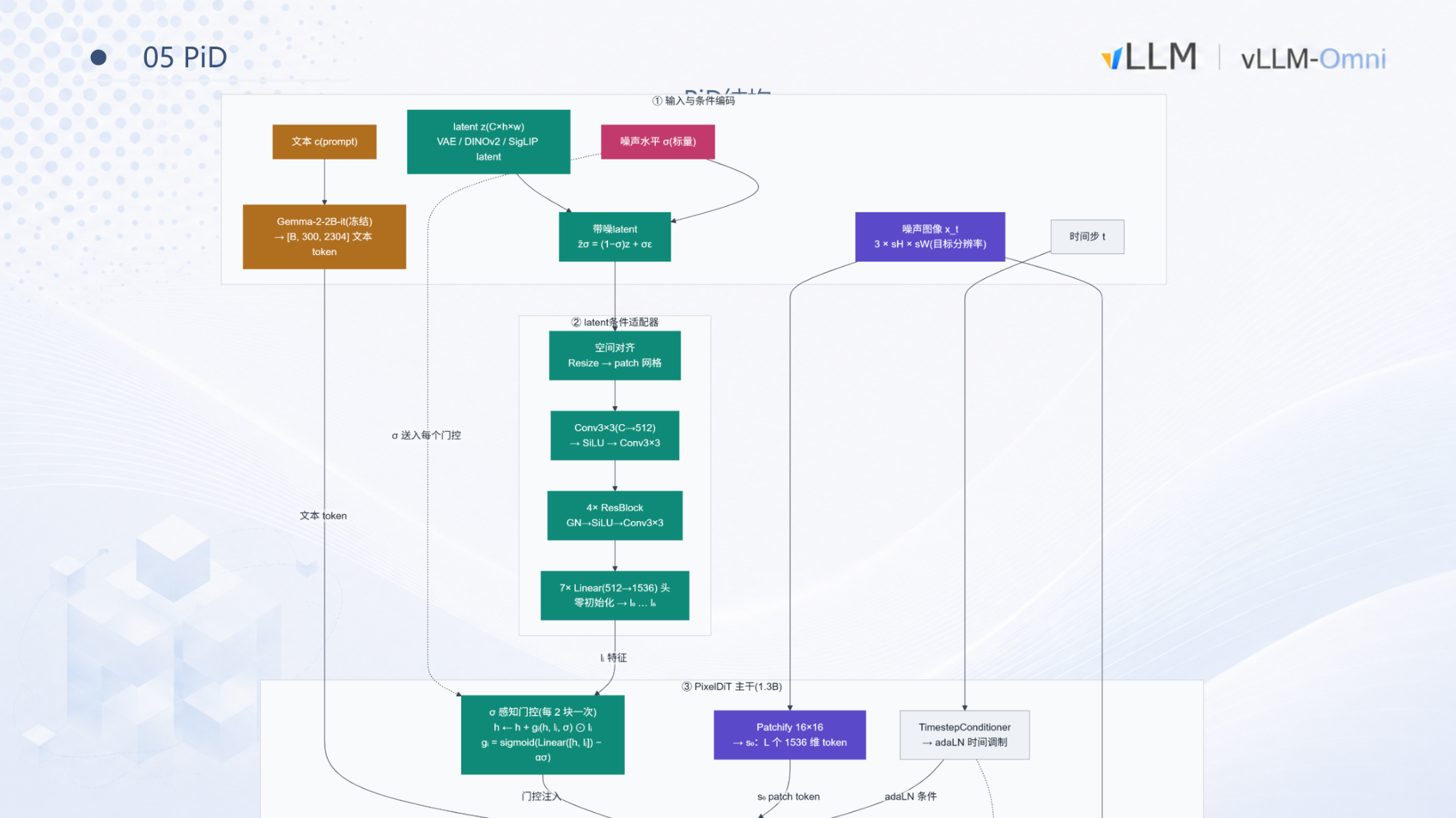Caption: PiD module structure and data flow. Source: presentation slide 11.

The figure shows three input paths and one backbone network:

1. Latent input (left): The intermediate latent from the main model's denoising process. It first passes through a condition adapter (latent condition adapter), composed internally of Resize → Conv3×3 → ResBlock → Linear, which converts the main model's latent representation into a feature format the PixelDiT backbone can consume. The condition adapter is the only part of PiD tightly coupled to the main model—swapping the main model requires retraining the adapter, while the backbone can be reused.

2. Text embedding input (top): A frozen Gemma-2-2B model encodes the text prompt to produce text tokens. The role of the text information is to guide detail regeneration during upsampling—the small-resolution latent itself does not carry high-frequency details, so textures and edges after upscaling must be generated under text-semantic guidance.

3. Target-resolution noise image (right): PiD prepares a pure-noise image at the target output resolution. For example, if the main model denoises at 512×512 and PiD performs 4× upsampling, the noise image is 2048×2048.

All three streams converge into the PixelDiT backbone (~1.3B parameters), which denoises the target-resolution noise image via cross-attention to directly produce a high-resolution pixel image. PiD is not a simple interpolation; it is a diffusion model trained for super-resolution that performs denoising in pixel space (rather than latent space), thereby completely bypassing VAE decode.

Causal Chain

Small-resolution latent (e.g., 512×512)
  ↓  Condition adapter translation
Features readable by PixelDiT
  ↓  + Target-resolution pure noise (e.g., 2048×2048) + text tokens
Cross-attention denoising
  ↓
High-resolution pixel image (2048×2048)

Minimal Example: State Evolution from 512 → 2048

Taking 4× upsampling as an example, assume the main model's total denoising step count N = 20:

Step	Location	Resolution	Notes
Steps 0–17	Main model DiT	512×512 latent	Runs in batch mode, enjoying high throughput
Step 18 (i.e., N−2)	Main model → PiD	—	Early termination; latent passed to PiD
PiD multi-step denoising	PixelDiT	2048×2048 pixels	Generates high-resolution result on the target-resolution noise image

The main model skips 2 denoising steps and operates entirely at small resolution throughout; the high-resolution generation cost is offloaded to the much lighter PiD.

Model Size and Boundaries

According to the speaker's oral estimate, the PiD backbone plus text encoder together total under 3B parameters, with a memory footprint far smaller than the main model. PiD supports 4× and 8× upsampling ratios. However, note the following:

• PiD denoises in pixel space; at very high target resolutions its own memory consumption also grows significantly.
• The condition adapter is coupled to the main model; after swapping the main model, the adapter must be retrained while the PixelDiT backbone remains unchanged.
• The presentation materials did not provide quality or performance data at larger upsampling ratios.

Summary: By decoupling high-resolution generation from VAE decode and delegating it to a lightweight pixel-space super-resolution diffusion model, PiD enables the main model to run batch inference on small-resolution latents. Next, we examine its resource savings and quality performance in actual deployment.

---

7 Performance and Limitations: PiD's Engineering Gains and Application Scenarios

Core question of this section: How much resource savings does PiD actually deliver for 2048-resolution image generation tasks? Do these gains come at the cost of image quality?

Measured Data at 2048 Resolution

The figure below contains quantitative comparisons of PiD across three dimensions—memory, latency, and quality—to assess its engineering viability:

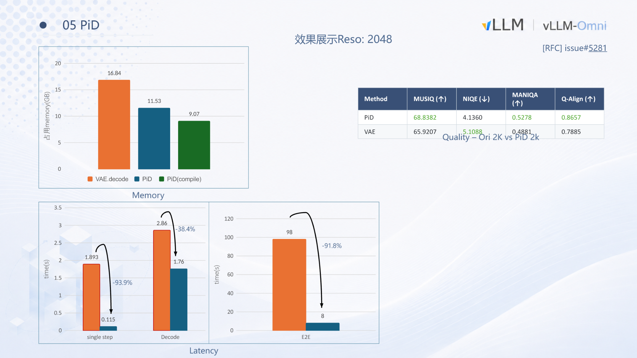Caption: PiD results—quantitative comparison of memory usage, latency, and image quality. Source: presentation slide 12.

Memory Usage

Approach	Memory (GB)	Savings vs. VAE decode
VAE decode	16.84	—
PiD	11.53	≈ 5.3 GB (~31.5%)

PiD runs the actual denoising on an input latent at 512 resolution, resulting in significantly smaller intermediate activations.

Latency Performance

• Per-step latency drops by approximately 93.9%—the input is only 512-resolution, so the per-step compute is roughly 1/16 of the original (quadratic reduction with resolution).
• End-to-end latency decreases by approximately 91.8%—combining the reductions in both denoising and decoding stages, the overall time is less than one-tenth of the original.

The presentation materials did not specify the exact GPU model or batch size configuration for these tests; percentage changes are more informative than absolute values.

Causal Chain

Input latent resolution reduced from 2048 to 512
  → Intermediate activation tensors shrink dramatically
    → Memory drops ~5 GB, per-step latency drops ~94%
  → Decoding switches from VAE convolutions to lightweight diffusion
    → Total end-to-end latency drops ~92%

Image Quality: Mixed Results

The slides provide a comparison across four no-reference image quality metrics:

Metric	PiD	VAE	Winner	Meaning
MUSIQ ↑	68.84	65.92	PiD	Multi-scale perceptual quality
NIQE ↓	4.14	5.11	PiD	Natural scene statistics deviation; lower is better
MANIQA ↑	0.528	0.488	PiD	Multi-dimensional attention-based quality
Q-Align ↑	0.866	0.789	PiD	Alignment quality score

PiD is slightly superior across all four quantitative metrics. However, the speaker explicitly noted: in terms of subjective visual perception, the two approaches each have their strengths. For example, VAE decode sometimes produces finer texture quality in certain scenes, while PiD sometimes delivers more vivid colors but occasionally exhibits stitching artifacts in fine details. Because PiD fundamentally "generates high resolution from low resolution," it inherently performs a degree of detail regeneration, and text-embedding control over the newly added details is not perfect. PiD is not a lossless replacement; in scenarios with strict image fidelity requirements, case-by-case evaluation is necessary.

Three Key Application Scenarios

Scenario	Key constraint	PiD's role
Edge-device inference with limited hardware	Single card with only 24 GB or 48 GB of memory	Reduces the memory of a 2048-resolution task to ~11.5 GB, making it feasible on consumer-grade GPUs
Small-shape batching for throughput	Server-side throughput maximization	Uses a smaller latent shape for batching, achieving higher GPU utilization
Ultra-high-resolution image generation	4K/8K output required	Leverages 4× and 8× upsampling to output ultra-high-resolution images without exceeding memory limits

In edge-inference scenarios, the 16.84 GB peak memory of traditional VAE decode nearly fills the usable space of a 24 GB GPU. Switching to PiD frees enough room to accommodate a medium-scale language-vision backbone.

---

Conclusion and Limitations

Core Conclusions

1. Asynchronous request dispatch is the cornerstone of all batching optimizations. Refining the scheduling granularity from entire requests down to individual denoising steps allows DiffusionEngine to dynamically insert or terminate requests in the gap between every step, with native support for interrupts and streaming of intermediate results.

2. The CPU overhead of dynamic batching is negligible. make_batch takes < 1 ms, compared to 1,000–1,200 ms for a single GPU step—three orders of magnitude apart.

3. Batching yields significant gains at small resolutions but limited gains at large resolutions. At 512×512 with BS=8, throughput improves by ~45% and latency drops by 33 seconds (of which 34% is attributable to amortized operator dispatch overhead); at 1024×1024 the improvement is less than 4%, as compute is already saturated.

4. Heterogeneous resolutions can be mixed-batched via GCD-based equal-length chunk splitting. Only self-attention requires special treatment (Recover-Scatter or varlen mask); all other operators execute in parallel at chunk granularity.

5. PiD trades minimal quality fluctuation for enormous resource savings. At 2048 resolution, memory drops from 16.84 GB to 11.53 GB and end-to-end latency decreases by 91.8%, providing a low-latency, low-memory pathway for edge-device inference and ultra-high-resolution generation.

6. PiD's core value lies in decoupling the main model's inference resolution from the output resolution. The main model always performs efficient batch inference on small latents, while high-resolution generation is handled by a lightweight super-resolution module with fewer than 3B parameters.

Explicit Limitations

• Limited batching gains at large resolutions: At 1024×1024 and above, compute is already saturated and batching cannot unlock further headroom. Beyond concurrency of 5, gains enter a plateau.
• Same-shape + same-CFG constraint: Requests with different resolutions or different guidance scales cannot be merged, limiting the size of the batchable request pool in practice.
• PiD image quality is not lossless: PiD leads on quantitative metrics, but subjective assessments vary by scene, with occasional stitching artifacts or overexposure tendencies in fine details.
• Condition adapter is tied to the main model: Each time the main model is swapped, PiD's condition adapter must be retrained.
• Single hardware baseline: All performance data in this article are based on the Qwen-Image model tested on a single Ascend A3 card; saturation points and gain curves may differ significantly on other hardware platforms.
• PiD's own memory scaling: PiD denoises in pixel space; whether PiD's own memory consumption at very high target resolutions can be further optimized through batching remains to be validated.