Reinforcement Learning Post-Training for Large Models: How RL-Kernel Completely Eliminates Train–Inference LogP Discrepancy

Source video: Bilibili BV1Ech96cEzW · Slides: RL-Kernel v0.1.0 slides

A Complete Engineering Guide from Low-Level Operator Reduction to Zero Mismatch Across Two Platforms

A hidden pitfall in reinforcement learning post-training for large models is that the log-probabilities (LogP) computed during the generation phase and the training phase are not numerically equal—even when the weights and inputs are identical. The source of the discrepancy is not model parameters but rather subtle differences in GPU floating-point reduction order between the two execution engines. Once amplified by the importance ratio, this last-bit deviation is sufficient to prematurely trigger gradient clipping, ultimately undermining training stability. The RL-Kernel project tackles this at the operator level, establishing strict numerical contracts for five classes of critical reduction operations. On both CUDA (H100) and ROCm (MI300X) platforms, it achieves zero discrepancy over 200 training steps with a Qwen3-8B Dense model, without sacrificing end-to-end performance. This article unfolds the complete technical details of this engineering effort layer by layer, following the chain of dependencies and causality.

Target audience: Senior algorithm engineers and systems engineers working on large-model reinforcement learning (RLHF/PPO), distributed training system development, operator optimization, and AI infrastructure.

Prerequisites:

• Familiarity with the basic workflow of reinforcement learning post-training for large models, including the alternation between Rollout and Training phases.
• Understanding of the basic concepts of Tensor Parallelism (TP) and Context Parallelism (CP) in distributed training.
• Foundational knowledge of GPU floating-point arithmetic characteristics, such as rounding errors and reduction operations.

Reading objectives:

1. Understand the low-level arithmetic root causes of the LogP discrepancy between the Rollout and Training phases.
2. Master the standardized preconditions and verification methodology for diagnosing numerical inconsistencies in distributed training.
3. Gain in-depth understanding of how RL-Kernel achieves strict numerical alignment by intervening in five classes of critical reduction operators.
4. Obtain the real-world engineering configurations and performance boundaries for achieving 200-step 0 Mismatch on both CUDA and ROCm platforms.

---

1. The Hidden Crisis in Reinforcement Learning Post-Training: LogP Discrepancy and Training Collapse

Same Model, Same Weights—Why Do Two Forward Passes Yield Different Results?

In the reinforcement learning (RL) post-training workflow, there is an easily overlooked prerequisite assumption: when the weights have not yet been updated, the Rollout phase (the RL phase that generates response tokens and records the initial log-probabilities) and the Training phase (the phase that recomputes log-probabilities and calculates the loss) should produce strictly identical log-probabilities (LogP, Log-Probability) for the same token.

The following table contrasts the key differences between the two phases:

Dimension	Rollout Phase	Training Phase
Execution engine	vLLM (high-performance inference engine, responsible for generating tokens and recording LogP)	Megatron-LM (distributed training framework, responsible for recomputing LogP and updating weights)
Input	Current weights + prompt	Same version of weights + full prompt and response tokens
Core computation	Token-by-token generation with LogP recording	Recomputation of selected-token LogP for the same batch of tokens
Output	rollout_logp	train_logp

Both sides describe the probability of the same policy, at the same moment, on the same token—logically, they must be equal. However, "same model" does not mean "same execution path." vLLM and Megatron-LM differ in the underlying kernel implementations they invoke, batch organization, tensor-parallel layout, and even floating-point reduction order, and these differences are sufficient to produce small but nonzero numerical discrepancies in LogP between the two sides.

How Discrepancy Progressively Destroys the Training Process

The figure below illustrates the complete causal chain from the emergence of discrepancy to the triggering of training collapse. The blue path represents the Rollout execution flow, and the orange path represents the Training execution flow; the two paths are connected at the same location by a red link marking the "first point of divergence"—the low-level operator bifurcation point. The right side annotates the downstream consequences of this divergence propagating along the computation graph.

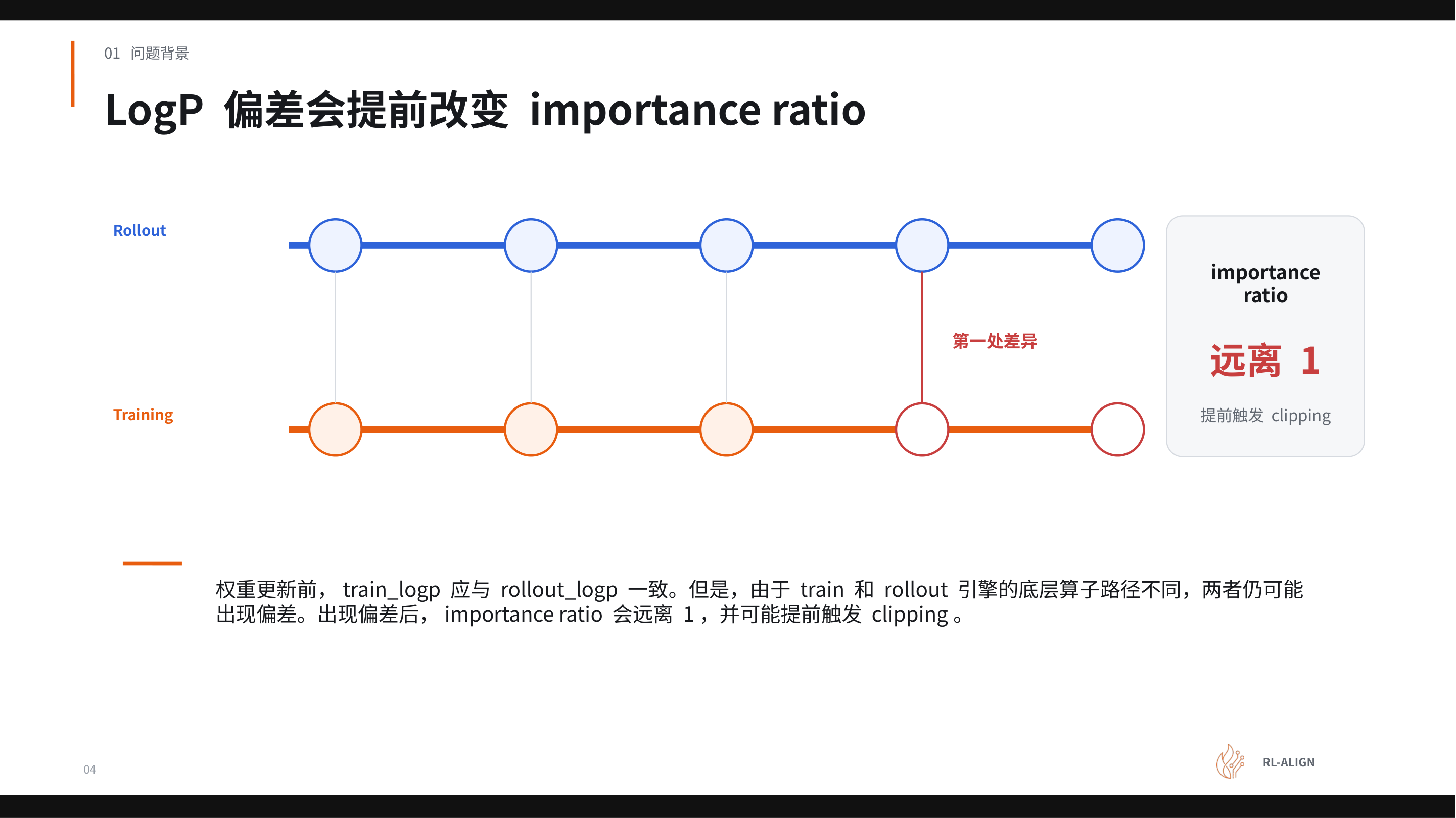Figure: Comparison of the Rollout and Training execution flows. Red links mark the positions where the two engines produce numerical divergence at the operator level and its downstream consequences. Source: Presentation slides, page 4.

Starting from the red-marked bifurcation point, the causal chain unfolds as follows:

1. Low-level operator path divergence → train_logp and rollout_logp exhibit a discrepancy Δ.
2. Importance ratio deviates from 1 — In policy gradient algorithms such as PPO: \(r(\theta) = \exp\!\bigl(\text{train\_logp} - \text{rollout\_logp}\bigr)\). When LogP values on both sides are strictly identical, \(r(\theta)=1\); once a discrepancy Δ exists, the ratio becomes \(e^{\Delta}\). Even if the per-token discrepancy is small, accumulation over many tokens in a long sequence can cause significant drift.
3. Premature triggering of clipping — The PPO clipping mechanism constrains \(r(\theta)\) to \([1-\epsilon,\;1+\epsilon]\) (where \(\epsilon\) is typically around 0.2). If Δ has already consumed part of the clipping headroom, the gradient signal from genuine policy improvement is prematurely truncated.
4. Training instability or collapse — The gradient signal is continuously suppressed, preventing the model from obtaining an effective update direction; in severe cases, training collapse occurs within hundreds of iterations, and the entire RL step is wasted, requiring a restart from a checkpoint.

Minimal Example: How a Single-Token Discrepancy Consumes Clipping Headroom

Consider a single-token example to appreciate the amplification effect: suppose rollout_logp = −2.300 and train_logp = −2.308 (a discrepancy of merely 0.008). Then \(r = \exp(-0.008) \approx 0.992\), still far from the clipping boundary.

However, in real-world scenarios, a single response may contain hundreds of tokens. If the discrepancy direction is consistent for every token—entirely plausible under a fixed operator path difference—the log-ratio accumulates linearly. Suppose each of 200 tokens has a discrepancy of 0.008; the cumulative log discrepancy reaches 1.6, and the ratio is approximately \(e^{-1.6} \approx 0.20\), which has far exceeded the \([0.8, 1.2]\) clipping interval, and the policy gradient signal is completely truncated.

Note: The numerical values above are intended solely to demonstrate the causal mechanism. The presentation materials did not provide precise statistics of actual discrepancies or quantitative measurements of clip ratios. Actual discrepancy magnitudes depend on model scale, sequence length, degree of parallelism, and the specific implementation of floating-point reduction.

Summary

Even in a single-machine single-GPU scenario, operator path differences are sufficient to introduce discrepancy; scaling to multi-machine multi-GPU settings, where tensor parallelism introduces changes in reduction order, further increases uncertainty. LogP consistency is not a soft metric where "close enough" suffices—it is a hard constraint that demands zero discrepancy (0 mismatch). Any systematic, however small, discrepancy will be amplified by the importance ratio, ultimately threatening the stability of the entire training pipeline.

The existence of the discrepancy is now established. The next step requires delving into the hardware and arithmetic levels to understand exactly at which stage of floating-point reduction these subtle differences are introduced.

---

2. The Physical Root Cause of Discrepancy: The Floating-Point Reduction Trap in GPU Parallel Computing

Same Inputs—Why Different Results?

The previous section confirmed that Rollout and Training exhibit last-bit numerical discrepancy in LogP for the same token. This discrepancy does not originate from model parameters or input data but rather from a frequently overlooked physical characteristic of how GPUs execute floating-point operations—floating-point reduction order: when multiple floating-point numbers need to be summed, different summation orders produce inconsistent results due to rounding at different positions.

Illustrated: Two Mathematically Equivalent Reduction Paths

The figure below uses the simplest structure to illustrate how reduction order changes floating-point output: the same four inputs, two different accumulation orders, two different results.

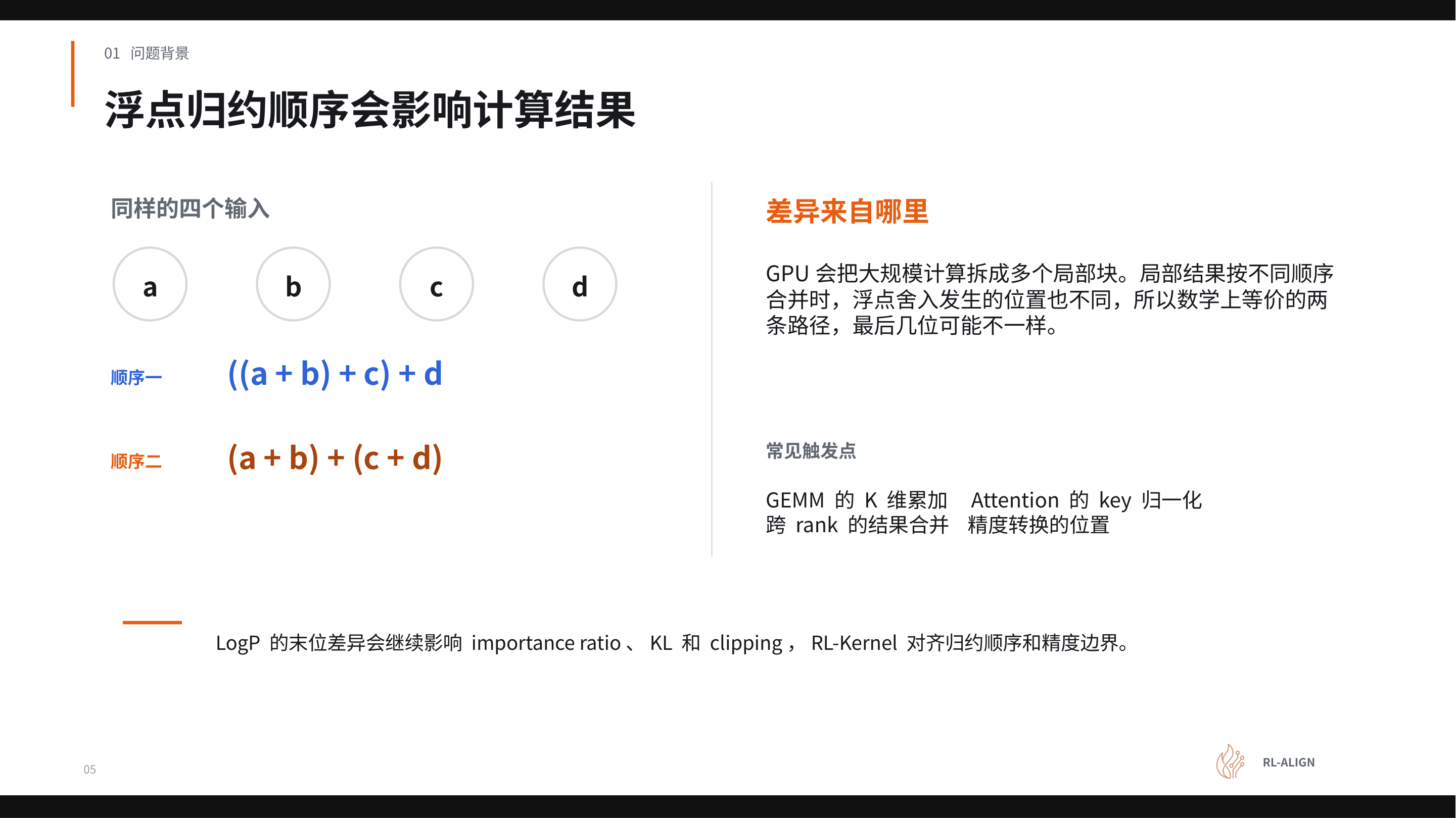Figure: Comparison of two reduction orders—Order 1 is a left-fold serial accumulation, and Order 2 groups pairs before merging. Source: Presentation slides, page 5.

The figure shows four inputs a, b, c, d and two paths:

Path	Expression	Accumulation steps	Intermediate roundings
Order 1	((a + b) + c) + d	3 serial additions	1 per step, 3 total
Order 2	(a + b) + (c + d)	2 parallel groups + 1 merge	3 total, but applied to different intermediate values

The two paths are perfectly equivalent in the real number domain, but under finite-precision floating-point representation, the position at which rounding occurs (i.e., which two numbers are added first) determines which last-bit information is discarded.

Causal Mechanism: From Block-Parallel Tiling to Last-Bit Discrepancy

When GPUs process large-scale matrix operations, they do not perform a single serial accumulation over the entire vector. Instead, the computation is split into multiple local blocks (tiles), each independently summed before merging. This process forms a three-step causal chain:

1. Tiling: In a single GEMM (General Matrix Multiply) operation, the K dimension—the dimension participating in the inner product—is partitioned into several segments assigned to different compute units.
2. Local reduction: Each compute unit completes accumulation within its own segment, producing a local partial sum. Each partial sum has already undergone its own rounding.
3. Global merge: The local partial sums are merged into the final result in a specific order. Different merge orders can produce different last-bit results.

The key insight is that even when computing the same operator, Megatron-LM and vLLM often choose different kernel implementations with different tile sizes and merge strategies—equivalent to making different choices between "Order 1" and "Order 2" in the figure above.

Four Common Trigger Points

The presentation materials explicitly listed four categories of computation most prone to reduction order divergence:

Trigger point	Reduction dimension / operation	Cause of divergence
K-dimension accumulation in GEMM	Inner product dimension K tiling size	Training and inference kernels select different tiles
Key normalization in Attention	Summation in the softmax denominator	Different chunking strategies due to Flash Attention version differences
Cross-rank result merging	Tensor Parallelism (TP) AllReduce	Multi-GPU reduction order depends on communication topology
Position of precision conversion	FP32 ↔ BF16 truncation point	Convert-then-accumulate vs. accumulate-then-convert

These four trigger points do not appear in isolation. A single forward pass involves dozens or even hundreds of operator invocations, each of which may introduce subtle differences at the last bit; these differences are amplified through nonlinear transformations in subsequent layers and ultimately converge in the LogP output.

From Single-GPU to Multi-GPU: What Does Parallel Scale Amplify?

In the single-GPU scenario, discrepancy arises only from tile reduction order differences within the kernel. When scaling to multi-GPU tensor parallelism, a new variable is introduced—the merge order of cross-rank AllReduce. Different TP degrees mean the same K dimension is split into different numbers of segments distributed across different GPUs; the tree or ring topology of AllReduce further alters the merge order of partial sums. Even if training and inference use the same number of GPUs, any difference in TP strategy or communication implementation can lead to inconsistent last-bit results.

Summary

Floating-point reduction order differences in GPU parallel computing are the physical root cause of last-bit discrepancies in train–inference LogP. This difference is not a bug but an inherent characteristic of finite-precision floating-point arithmetic under parallel tiling. To eliminate it, synchronizing weights alone is far from sufficient—one must also align accumulation order, computation precision, and the rounding positions of intermediate results. Before proceeding with per-operator fixes, a systematic diagnostic framework must first be established to clarify which preconditions must be aligned first.

---

3. Establishing the Diagnostic Baseline and System Panorama: The Synergy of vime and RL-Kernel

Where to Start When LogP Is Inconsistent?

When LogP discrepancy appears between the two sides, the most intuitive reaction is to suspect the underlying operators. But if the two sides have loaded weights from different training steps, or if the prompt–response concatenation boundary is off by one token, no amount of operator-level alignment will eliminate the difference. Therefore, diagnosis must proceed layer by layer: lock down external conditions first, then drill into internal computation.

Five Prerequisite Alignment Conditions

Before comparing any pair of LogP values, the following five baseline conditions must be confirmed item by item to all be consistent. If any single item is misaligned, the difference cannot be attributed to the computation path:

#	Condition	Specific content to verify
①	Weight version	Rollout and Training must correspond to the same checkpoint and the same training step
②	Input boundaries	Concatenation and truncation of prompt, response, target tokens, and active mask
③	Positional information	Position IDs, RoPE parameters, causal mask shape, KV visible range
④	Logical state	Token assignment across ranks, actual vocabulary range, tensor-parallel shard mapping
⑤	Stochastic conditions	Random seed and sampling state

Take condition ④ as an example: when TP is enabled, the logit vector of the same token is sharded across different GPUs. If the shard mappings are inconsistent between the two sides, even with completely identical weights, the probability values retrieved at the target token position will differ. Condition ⑤ follows the same logic—certain Dropout or sampling paths are controlled by the seed, and out-of-sync state introduces irreproducible noise.

Decision rule: Only after all five conditions pass can residual differences be traced downward to the numerical paths of the execution engines and operators.

System Panorama: Four-Layer Architecture and Responsibility Boundaries

Determining who locks down external conditions and who aligns internal computation requires a system-wide architecture diagram. The figure below shows the four-layer dependency relationship from the scheduling framework to the hardware backend, with RL-Kernel inserted as an independent operator layer—the critical position for eliminating numerical discrepancy.

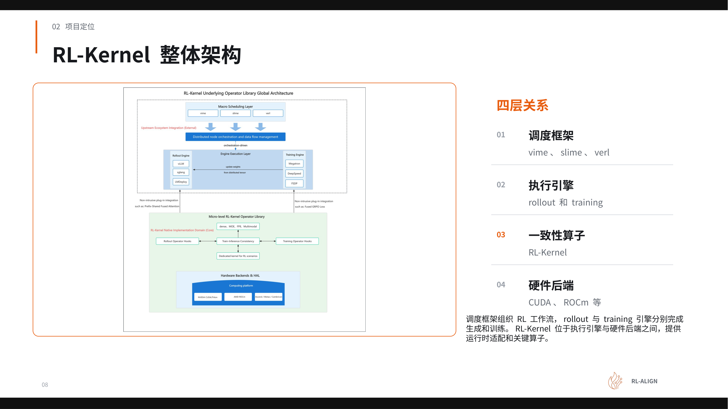Figure: RL-Kernel overall architecture. The four layers from top to bottom are the scheduling framework, execution engines, the RL-Kernel operator layer, and the hardware backend. Source: Presentation slides, page 8.

The four layers form a clear dependency relationship from top to bottom:

1. Scheduling Framework Layer — Includes vime (a scheduling framework responsible for orchestrating the RL workflow timing, data flow closure, and weight synchronization). This layer determines when to do what: first Rollout generation, then Reference scoring, then Actor training, and finally synchronizing the updated weights back to the inference side.
2. Execution Engine Layer — The Rollout side uses vLLM, and the Training side uses Megatron-LM. The two engines each have their own independent batch organization, parallelism strategies, and kernel scheduling logic.
3. Consistency Operator Layer (RL-Kernel) — Situated between the execution engines and the hardware backend, providing runtime adaptation and critical operator replacement.
4. Hardware Backend Layer — Such as CUDA, ROCm (AMD's hardware backend computing platform), etc. Different backends may exhibit differences in floating-point rounding behavior and kernel implementations; RL-Kernel must shield these differences downward.

The arrow directions reveal the causal chain: the scheduling framework dispatches tasks and data to the execution engines → the execution engines invoke operators provided by RL-Kernel → RL-Kernel maps computation instructions to the specific hardware backend. Information flows unidirectionally, and responsibilities do not overlap.

The division of labor between the two core components can be summarized in one sentence: vime ensures both sides process the same batch of data at the same moment; RL-Kernel ensures both sides compute the same LogP for that batch of tokens.

Dimension	vime's responsibility	RL-Kernel's responsibility
Level of concern	Macro-level timing and data flow	Micro-level numerical computation
Core actions	Organize execution order; record weight versions; complete the sampling–training–update–sync closed loop	Define arithmetic contracts (normalization range, mask positions, LogP computation definition); restore token logical order; fix cross-rank merge order; constrain precision conversion boundaries
Alignment conditions covered	① Weight version ② Input boundaries ⑤ Stochastic conditions	③ Positional information (partial) ④ Logical state + all operator-level precision rules

RL-Kernel refers to its operator-level rules as Numerical Contracts—explicitly codifying the computational details prone to train–inference divergence so that both engine sides must execute according to the same specification. The contracts cover four categories: arithmetic definitions, token ordering, result merging, and precision boundaries.

Summary

The five prerequisite conditions are mandatory checkpoints in the diagnostic process; skipping any one of them may lead to misdiagnosis. vime and RL-Kernel are complementary and non-overlapping: the former controls external variables (timing, data, weights), while the latter controls internal computation rules (arithmetic, ordering, merging, precision). This section has narrowed the diagnostic space from "the entire system" down to "RL-Kernel's four categories of numerical contracts." The next section delves into the internals of RL-Kernel, dissecting how it fulfills these contracts on each critical operator.

---

4. Core Mechanism Analysis: Alignment of Five Classes of Reduction Operators and Global Statistics

Why Reduction Operations Become the Entry Point for Discrepancy

In the forward computation of large models, nearly every layer involves a reduction operation—an operation that merges multiple local values along a certain dimension into a single global result, such as summation or taking the maximum. When Megatron-LM and vLLM use different kernel implementations, different tiling strategies, or different precision conversion positions, even with identical inputs, the intermediate values and final outputs of reductions may diverge at the last significant digit. These divergences propagate layer by layer through the network and ultimately accumulate in the selected-token LogP.

The core task of RL-Kernel v0.1.0 is to identify and lock down all reduction paths that affect LogP so that the two engines produce consistent results for the same batch of tokens.

Panorama: Five Classes of Reduction and Their Dimensions

RL-Kernel v0.1.0 categorizes the computations affecting the final LogP into five classes of reduction operators, each merging local results into global results along a different dimension:

Class	Reduction dimension	Typical source of divergence
RMSNorm	hidden dimension	Mean and variance depend on the accumulation order along the hidden dimension
Attention	visible key range	softmax depends on the local maximum and exponential sum over visible keys
GEMM / SwiGLU	K dimension	Different tile partitions alter local accumulation and merge patterns
Linear LogP	vocabulary	LogSumExp requires normalization over the full vocabulary
Collectives	cross-rank	Merge order of cross-GPU results affects last-bit precision

All five classes share a common pattern: partition data → local computation → merge results. Whenever the number of partitions, merge order, or intermediate precision is inconsistent between the two sides, the difference enters the final LogP.

Focus: The Shared Dependency of Attention and Linear LogP on LogSumExp

Among the five classes of reduction, Attention and Linear LogP are particularly critical because they share the same type of core statistic—LogSumExp (LSE)—the global statistic required to convert a set of raw scores into normalized probabilities, defined as:

\[\text{LSE}(x_1, \dots, x_n) = \log\!\Bigl(\sum_{i=1}^{n} e^{x_i}\Bigr)\]

In practice, for numerical stability, the local maximum \(m = \max(x_i)\) is first subtracted, and then \(m + \log\sum e^{x_i - m}\) is computed.

The figure below shows the shared dependency structure of the two computation paths on LSE. The left Attention branch reduces over visible keys, the right Linear LogP branch reduces over the full vocabulary, and the central node labels the LSE statistic type they share.

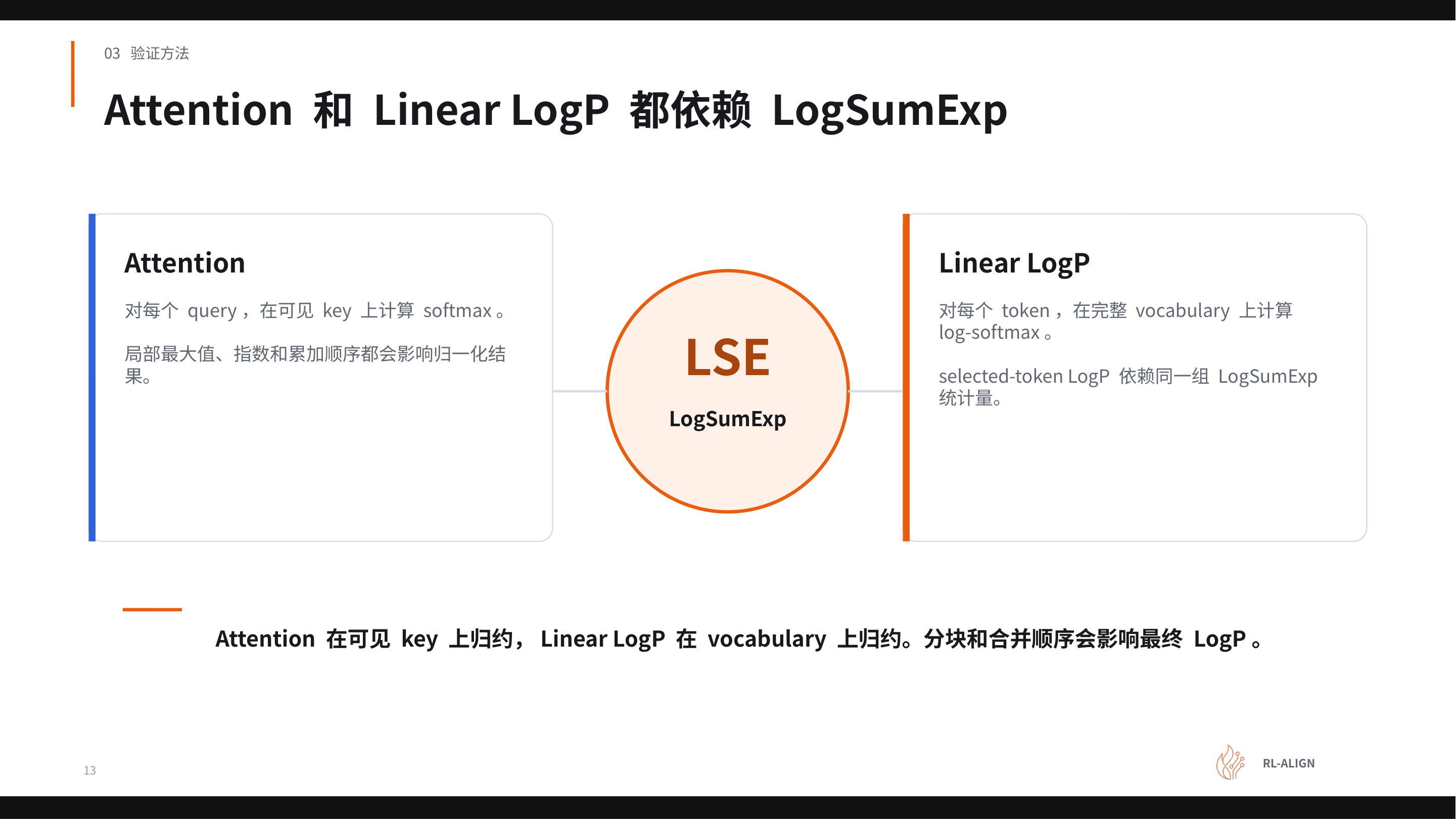Figure: The left Attention branch computes softmax for each query over visible keys; the right Linear LogP branch computes log-softmax for each token over the full vocabulary; the central LSE node indicates the LogSumExp statistic type shared by both. Source: Presentation slides, page 13.

Each of the three regions in the figure carries distinct information:

• Left Attention box: A single query scores multiple keys simultaneously, and all scores must undergo softmax jointly over the complete range of visible keys. The local maximum and the order of exponential accumulation directly affect the normalization result.
• Right Linear LogP box: The model scores the entire vocabulary, then obtains the log-probability for each token via log-softmax. Even if only a specific selected token is of interest, its LogP still depends on the LSE computed from scores across the entire vocabulary—changes in scores at other positions also alter the target probability.
• Central LSE node: The confluence point of the two paths. Attention reduces along visible keys and Linear LogP reduces along the vocabulary, but the mathematical structure of the LSE computation is identical, so they face the same type of consistency risk.

Causal Chain: How Block Merge Order Alters LSE

After the vocabulary or key sequence is partitioned across multiple blocks (or multiple GPUs), each block independently computes a local maximum \(m_j\) and a local exponential sum \(s_j\). The standard procedure for merging two blocks of LSE is:

\[m = \max(m_1, m_2),\quad s = s_1 \cdot e^{m_1 - m} + s_2 \cdot e^{m_2 - m}\]

Floating-point arithmetic does not satisfy the associative law, so the merge order affects the result. Consider three blocks as an example: Engine A first merges blocks 1 and 2, then merges with block 3; Engine B first merges blocks 2 and 3, then merges with block 1. During the two merge processes, the exponential difference \(e^{m_j - m}\) values differ, and the rounding positions of BF16 or FP32 truncation also differ, so the final LSE can diverge at the last bit. This divergence is amplified after softmax normalization and directly manifests in the selected-token LogP.

RL-Kernel's countermeasure is: strictly prescribe the tiling strategy and merge order, and explicitly define the step boundaries for FP32 accumulation and precision conversion positions, so that both engines maintain identical local maximums, exponential sums, and rounding behavior at every step.

Multi-GPU Extension: Additional Variables Introduced by Collectives

When TP or CP (Context Parallelism) is used, the reduction scope of a single operator spans multiple GPUs, and Collectives become the fifth class of operations that must be aligned. Note that even if the communication layer itself is deterministic, if the local results fed to the communication layer from each GPU already differ, the global result after communication will also differ—the root cause lies upstream, not in the communication itself. Furthermore, when batch size, sequence length, and degree of parallelism change, the system may select different kernel paths, and both the number of partitions and the merge order change accordingly, requiring re-verification of alignment status.

Summary

Controlling the consistency of global statistics—especially LSE—is the key lever for eliminating train–inference LogP discrepancy. RL-Kernel v0.1.0 locks down the complete critical path affecting LogP under a unified tiling strategy, merge order, and precision boundary by covering five classes of reduction: RMSNorm, Attention, GEMM/SwiGLU, Linear LogP, and Collectives. With the mechanism design in place, the immediate next question is: how can one systematically verify that these alignment modifications have indeed eliminated the discrepancies?

---

5. Verification Methodology: Stripping Stochasticity and Precise Layer-by-Layer Localization

Why Are Discrepancies in Online Training Hard to Reproduce?

Every step of RL online training involves sampling—different random seeds generate different token sequences, causing the inputs between Rollout and Training to vary inherently. When inputs are inconsistent, even if operator-level numerical discrepancies exist, they are completely drowned out by sampling stochasticity, and the engineer cannot determine whether a subtle LogP difference originates from the operator implementation or from input differences.

This creates an engineering contradiction: finding a static operator defect within a dynamically changing online environment. The solution is to first freeze the dynamic factors and then systematically diagnose layer by layer under deterministic conditions.

Four-Step Verification Process

The figure below presents the complete closed-loop process from locking inputs to returning to online training. The highlighted node marks the location of the "first divergence"—the core target of the entire diagnostic process.

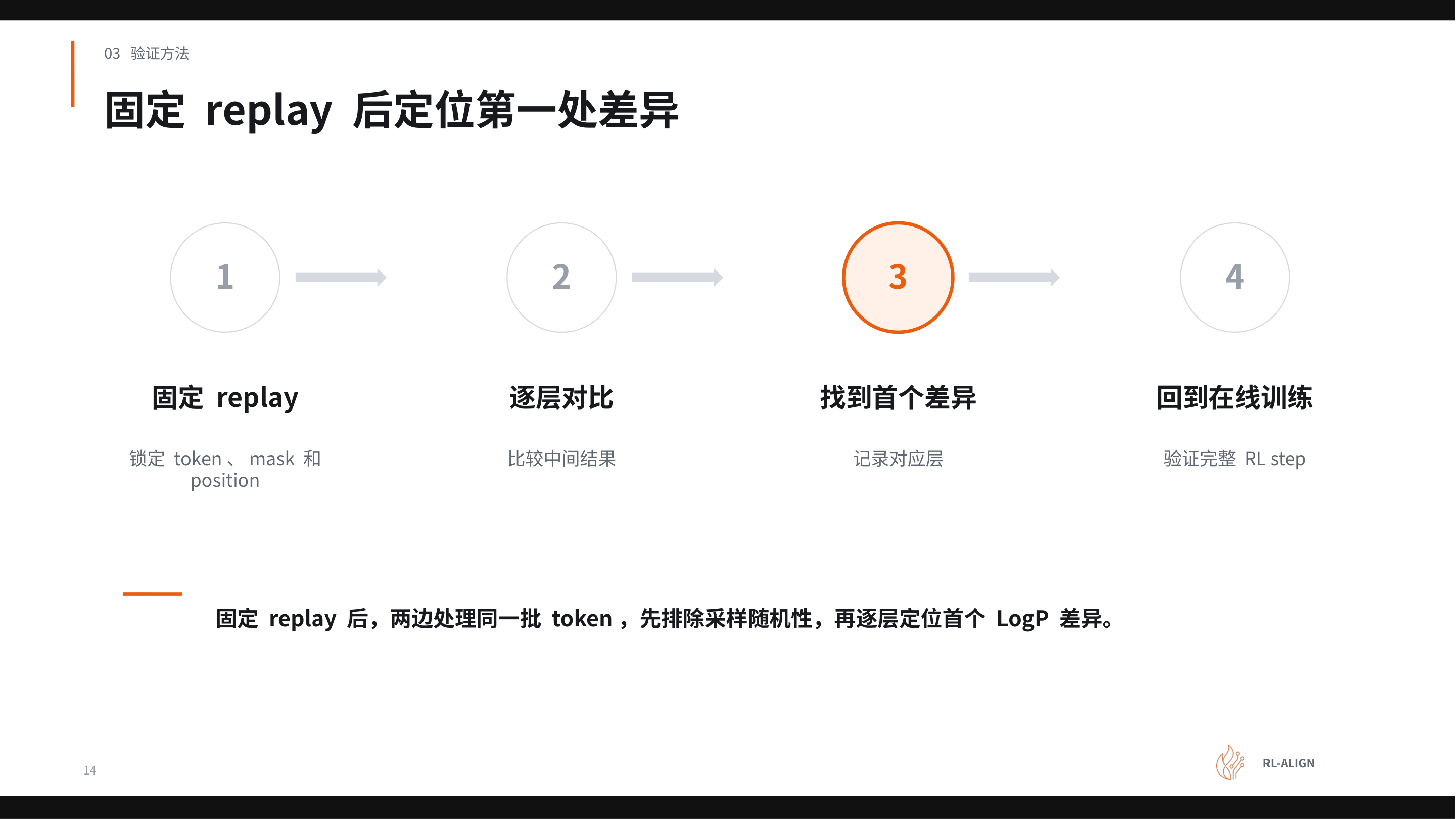Figure: Four-step verification process—a closed loop from locking inputs to returning to online training. The highlighted circled node marks the first divergence point. Source: Presentation slides, page 14.

The four numbered nodes in the process diagram have the following meanings:

Step	Action	Purpose
① Fix replay	Lock tokens, masks, and positions	Eliminate sampling stochasticity so both sides process the same batch of inputs
② Layer-by-layer comparison	Compare the intermediate tensor output of each layer	Narrow the diagnostic scope
③ First divergence	Record the first layer where inputs are identical but outputs differ	Precisely locate the root-cause operator
④ Return to online training	Run a complete RL step after the fix	Confirm the fix is equally effective in the dynamic environment

Why Find the "First" Divergence?

The core logic of layer-by-layer comparison is causal inheritance: if the output of layer \(k\) has already diverged, then even if layer \(k+1\) is implemented perfectly correctly, its output will also differ because it inherits the error from the previous layer. Therefore, only by finding the first divergence point—the first operator layer where the inputs are identical but the outputs differ—can one avoid spending significant time on downstream "inherited" differences. After finding that layer, one must further inspect its internal precision, reduction order, kernel selection, and other factors.

The Absolute Consistency Requirement

A critical engineering judgment criterion is: comparison results must be perfectly identical, not merely within some extremely low error tolerance. Even if the per-layer error is minuscule, after propagating through dozens of forward computation layers, the error accumulates layer by layer and is further amplified with increasing token sequence length. This criterion equally covers communication stages—the computation results from each partition must be accumulated in a fixed order to guarantee determinism in cross-GPU scenarios.

The Closed Loop from Fixed Replay to Full Online Verification

After fixing an operator, the process is not complete. One must re-execute the fixed replay to confirm that the divergence at that layer has been eliminated and no new divergence points have been introduced, and only then return to the online training environment for end-to-end validation. The above process can be summarized as a closed loop:

1. Freeze inputs → Fixed replay eliminates sampling variables
2. Narrow scope → Layer-by-layer comparison to find the first divergence layer
3. Fix operator → Make corrections to precision, reduction order, or kernel selection
4. Regression verification → First confirm the fix under fixed replay, then return to online training for full-process validation

Summary

The applicability of this methodology presupposes the ability to save and replay a fixed batch of weights, tokens, and masks. In scenarios with extremely large models or complex cross-node communication paths, the storage overhead of saving complete intermediate tensors also needs to be taken into account—the presentation materials did not provide specific storage overhead figures. Fixed replay is the critical step in transforming the problem from irreproducible to reproducible; layer-by-layer comparison and first-divergence localization reduce diagnostic complexity from the entire model to a single operator; the absolute consistency criterion eliminates the risk of error accumulation. This process constitutes a reusable, standardized diagnostic methodology for numerical consistency.

---

6. Benchmark Validation: 0 Mismatch and Performance Preservation on the CUDA Platform

The Engineering Tension: The Seesaw Between Precision Alignment and Training Throughput

The previous sections established the complete technical approach for eliminating train–inference LogP discrepancy. Now two core questions arise: can these alignment mechanisms deliver on the "zero error" promise on a real GPU cluster? And do the constraints imposed to guarantee determinism—such as fixing reduction order—significantly slow down end-to-end training speed? A natural tension exists between the two: tightening floating-point accumulation paths typically means sacrificing parallelism, while relaxing constraints introduces uncontrollable numerical discrepancy.

Experimental Configuration

The experiment used a Qwen3-8B Dense (a dense model architecture in which all parameters participate in computation during every forward pass, as opposed to MoE architecture) model, running on a single node with 8 × NVIDIA H100 80 GB:

Configuration item	Value
Model	Qwen3-8B Dense
Hardware	1 node, 8 × H100 80 GB
Parallelism strategy	TP4 / CP2
Global batch	128
Random seed	1234
Number of steps	200

The control group used the native vime path, and the experimental group used RL-Kernel + vime. Both groups used completely identical model weights, training data, and hyperparameters.

Key caveat: The presenter explicitly noted that performance is strongly workload-dependent—increasing the batch size or lengthening responses changes the ratio of computation to communication time. The conclusions below cannot be directly extrapolated to other configurations.

Core Result: Zero Discrepancy Across All 200 Steps

The figure below uses two sets of line charts to compare the LogP consistency performance of the native vime path (red line) and the RL-Kernel path (blue line) across 200 RL steps. The left chart shows the number of mismatched tokens, and the right chart shows the maximum absolute LogP difference.

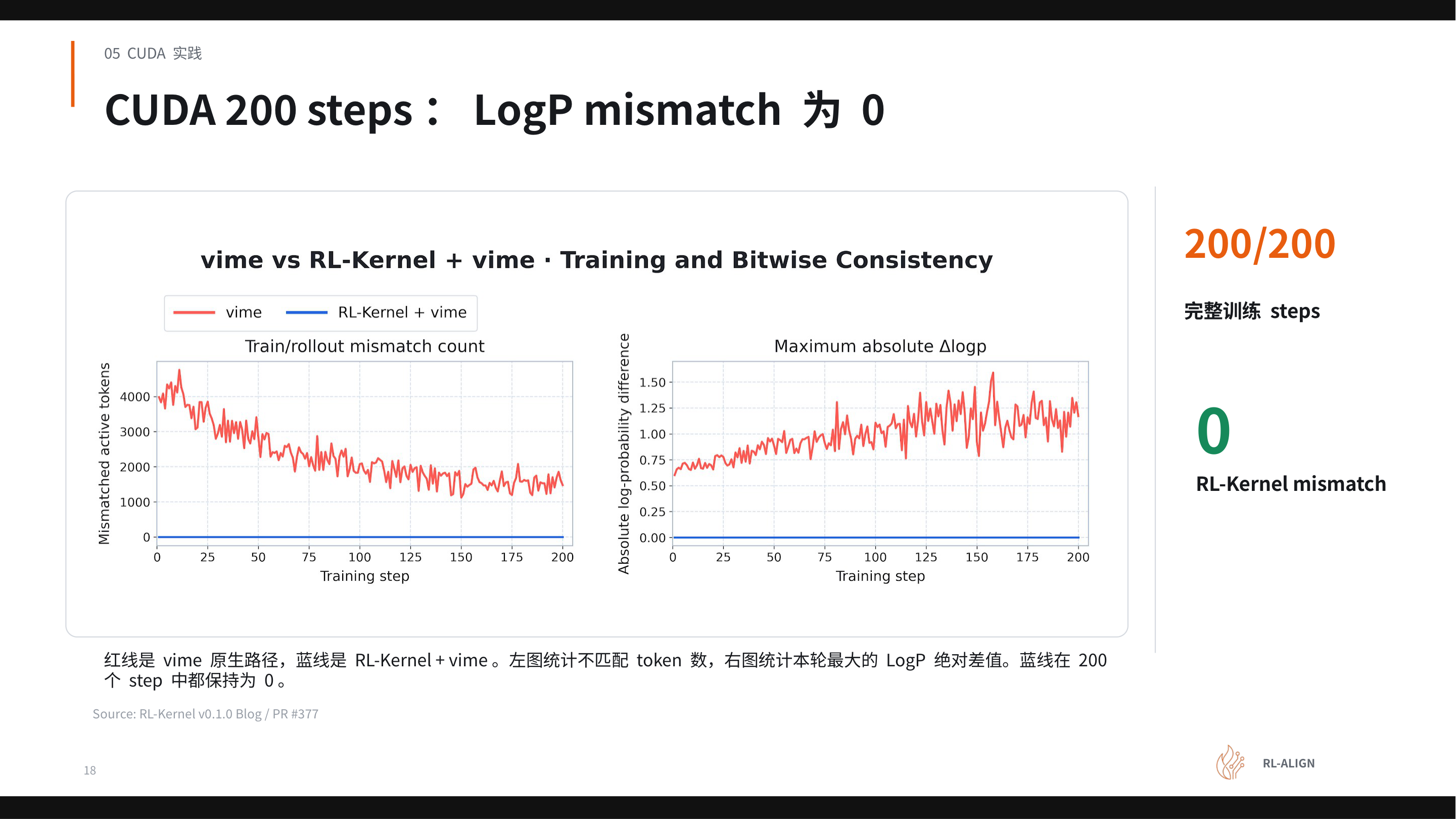Figure: LogP mismatch tracking curves over 200 RL steps on the CUDA platform. The red line represents the native vime path, and the blue line represents the RL-Kernel + vime path. Source: Presentation slides, page 18.

The horizontal axis of both line charts is the training step (0–200):

• Left chart—Number of mismatched tokens: The red line fluctuates violently between 0 and approximately 4,000, indicating that thousands of tokens in each batch may have inconsistent probability signals between training and inference. The blue line sits on the zero line from step 1 onward, with no elevation across all 200 steps.
• Right chart—Maximum absolute LogP difference: The red line oscillates continuously in the 0.25–1.50 range, meaning that the maximum per-token discrepancy can exceed 1.0. The blue line is likewise identically zero.

Both charts jointly confirm: under the given configuration, RL-Kernel achieved 0 mismatch across 200/200 steps—not a single token's LogP exhibited train–inference inconsistency. The fluctuation magnitude of the red line also inversely illustrates the severity of the problem: discrepancies spanning thousands of tokens are sufficient to distort the policy gradient direction.

Performance Preservation: Offsetting Alignment Constraints with Computation Fusion

Locking deterministic floating-point paths would theoretically reduce throughput. RL-Kernel employs six targeted optimizations to keep end-to-end performance essentially on par with the native vime path:

#	Module	Alignment constraint	Performance compensation mechanism
01	GEMM	Auto-selects cuBLASLt no-split-K or SM90; SM90 assigns a single CTA to each output tile, accumulating along the full K dimension in a fixed order	Fixed reduction eliminates nondeterminism; saves the extra synchronization of split-K
02	RMSNorm	Switched to torch RMSNorm to unify normalization semantics	Eliminates implicit differences between different kernel implementations
03	Attention	FA4 strict core with split-K disabled; backward uses a deterministic path	Reuses FA4's existing deterministic kernel
04	FFN	Packed gate/up, SwiGLU, and down GEMM executed in separate stages	Reuses packed weights, reducing memory movement
05	LM head / LogP	Both Training and Rollout reuse local logits	Eliminates redundant LM-head GEMM, yielding a net positive gain
06	CUDA IPC communication	Single-node fixed-tree collective; TP1/2/4/8 all use a fixed balanced tree, locking data types and first-entry position	Fixed tree topology eliminates communication order nondeterminism while maintaining low IPC latency

The key causal logic is: alignment constraints impose restrictions on certain paths (e.g., disabling split-K), but they drive leaner implementations on other paths—the weight reuse in item 04 and the GEMM deduplication in item 05 are both instances of "streamlined by alignment" positive gains that offset the performance cost of determinism constraints.

Note: The presentation materials did not provide specific throughput numbers (e.g., tokens/s) or per-item latency breakdowns. "End-to-end performance on par with the native path" is a qualitative conclusion.

Summary

The applicability boundaries of this section's conclusions must be made explicit: the model covers only Qwen3-8B Dense and does not include MoE architecture; the scale is a single node with 8 GPUs, without testing multi-node cross-machine communication; the 200-step verification confirms short-term strict consistency, and performance over longer training durations was not disclosed in the current materials. Within these boundaries, the core conclusion holds: consistency and high performance are not mutually exclusive. By locking operator-level deterministic paths one by one and compensating overhead with computation fusion and fixed communication topologies, RL-Kernel demonstrated the engineering feasibility of a zero-discrepancy approach on the CUDA platform. The natural next question is: does this alignment logic remain effective when switching to a different hardware backend?

---

7. Cross-Platform Generalization: Bit-Exact Consistency on the ROCm Architecture

Is the Consistency Contract Tied to Specific Hardware?

The numerical contracts established on the NVIDIA H100 in the previous section—fixed accumulation order, locked reduction paths, unified precision conversion timing—are fundamentally constraints on floating-point arithmetic determinism. Once the hardware backend is changed, the instruction set, matrix compute units, and communication primitives all change, and every rule in the contract requires finding an equivalent implementation on the new platform.

Experimental Configuration

The validation experiment was conducted on a single node with 8×MI300X (192 GB HBM3 / GPU):

Dimension	Value
Model	Qwen3-8B Dense
Hardware	1 node, 8× MI300X 192 GB
Parallelism strategy	TP4 / CP2
Global batch	8
Random seed	1234

Important difference: The Global Batch on the ROCm side is 8, different from the 128 in the CUDA experiment, so the absolute runtimes on the two hardware setups cannot be directly compared across platforms.

Result: 9.4 Million Element-Wise Comparisons, Zero Discrepancy

The figure below presents the bit-exact consistency verification over 200 training steps on the ROCm platform. Focus on the comparison between the red line (native vime path) and the blue line (RL-Kernel path), as well as the total cumulative number of elements compared.

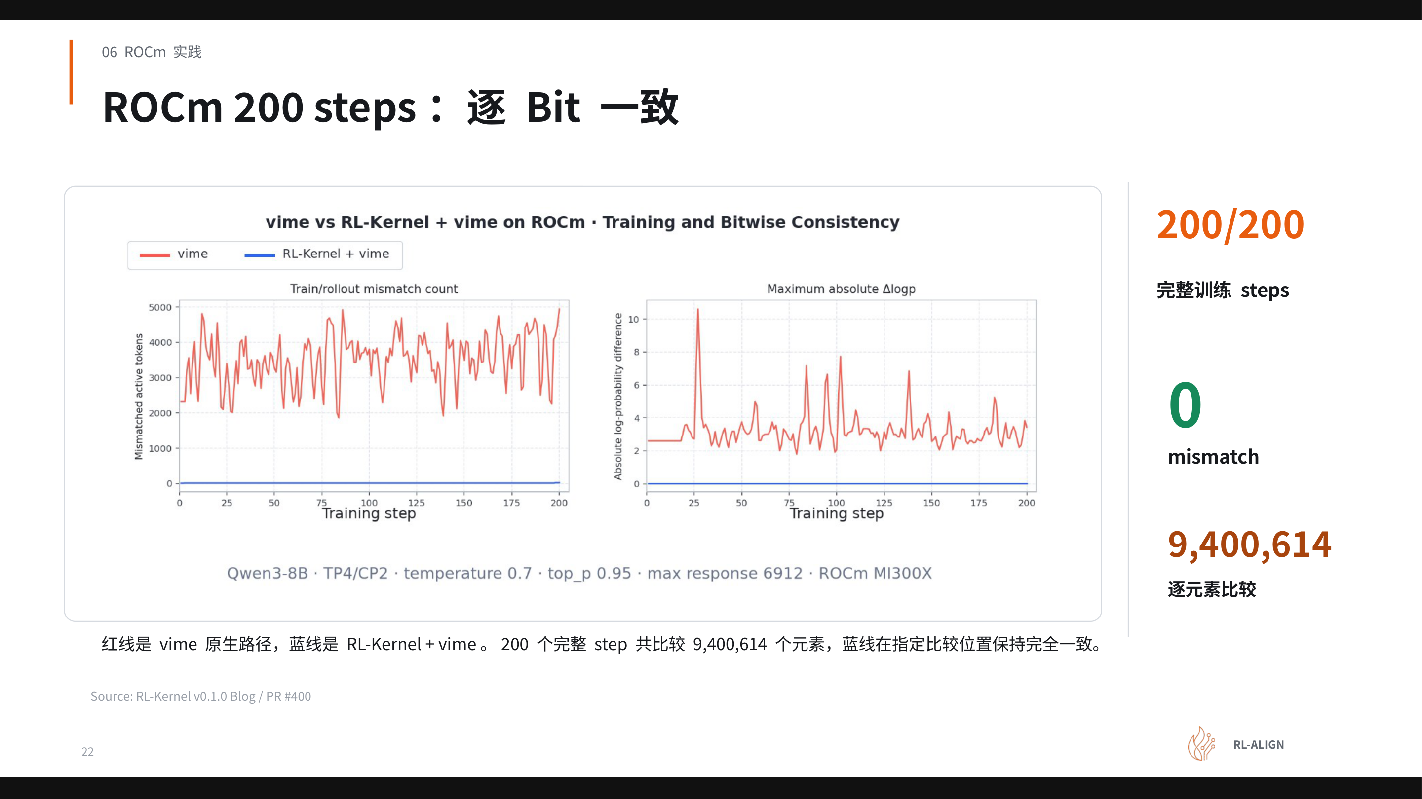Figure: Left chart shows mismatch count over training steps; right chart shows maximum absolute ΔlogP over training steps. The red line represents the native vime path, and the blue line represents the RL-Kernel + vime path. Source: Presentation slides, page 22.

Three elements in the figure are noteworthy:

1. Red line (native vime path): The mismatch count shows significant fluctuation across multiple steps, and the maximum absolute ΔlogP is likewise nonzero—a direct visual manifestation of numerical divergence when the two engines each execute independently.
2. Blue line (RL-Kernel + vime): Across all 200 training steps, it remains tightly on the zero line, with both mismatch count and maximum absolute ΔlogP at 0.
3. 9,400,614: The total number of element-wise comparisons accumulated over 200 steps. With nearly ten million floating-point value comparisons and zero deviation on the blue line, the consistency is not "statistically close" but strictly bit-exact.

Equivalent Implementations Across Six Modules

Zero discrepancy does not happen automatically. Each critical operator on the ROCm platform independently satisfies the numerical contract:

• GEMM: A custom MFMA (Matrix Fused Multiply-Add, AMD's matrix operation instruction) kernel with a fixed chunk order; intermediate results are merged at FP32 precision before being written back to BF16, ensuring a unique accumulation path.
• Attention default path: Uses the AITER/CK non-split strict core implementation; the paged decode phase uses a fixed CK path, eliminating nondeterminism from branch selection.
• Attention optional path: Triton-based chunked attention with fixed block partitioning, chunk order, and rescale merge order.
• FFN: Triton/MFMA strict GEMM implementation, executing packed gate/up, SwiGLU, and down projection sequentially in a fixed, non-interchangeable order.
• LogP: Each TP shard independently computes local statistics first, then merges in a fixed vocab tile order, preventing the reduction order from fluctuating with scheduling.
• Communication and execution: HIP IPC (Inter-Process Communication) handles small data transfers, and RCCL (ROCm Collective Communications Library, AMD's collective communication library) handles larger data transfers; locally, a fixed tree reduction is used, combined with HIP Graph and cache reuse to ensure a deterministic execution order.

These six rules correspond at the abstract level exactly to the contracts on the CUDA side—what changes are the underlying instructions and communication primitives; what remains invariant is the core set of invariants: "fixed accumulation order, fixed reduction path, locked precision conversion timing."

Under the 0 mismatch condition, RL-Kernel's end-to-end runtime on ROCm is essentially on par with the native vime path—consistency alignment did not introduce significant performance regression. However, it must be emphasized again: "on par" here is limited to a within-ROCm longitudinal comparison and cannot be used as a cross-platform conclusion against the CUDA side. The presentation materials did not provide specific runtime figures for a side-by-side comparison of the two platforms.

Summary

The current validation covers only a single configuration: the Qwen3-8B Dense model, single-node 8×MI300X, TP4/CP2; performance under larger scales or MoE architectures has not been publicly disclosed. Nonetheless, this set of experiments confirms a key judgment: the abstraction of the numerical contract is cross-hardware universal. As long as an equivalent implementation satisfying the contract is found for each operator on the new platform, bit-exact consistency can be transferred from one GPU architecture to another. With cross-platform verification complete, the next step is to objectively assess the limitations of the current version and plan the future evolution roadmap.

---

8. Engineering Boundaries and Evolution Roadmap: The Next Step from Dense to MoE

Problems Solved and Gaps Yet to Be Crossed

Eliminating train–inference LogP discrepancy reached a clear milestone in v0.1.0, but "zeroing out mismatch" is a means, not an end. The core tension is: numerical consistency has been proven achievable, but its actual impact on long-horizon RL training benefits still lacks sufficient evidence.

Dimension	Verified	Still needs verification
Numerical correctness	LogP mismatch is 0 within 200 training steps	Whether reward improves stably over longer training horizons (multiple seeds)
Hardware platforms	Dual-platform: CUDA and ROCm	Domestic backends (MUSA, Ascend) for end-to-end training
Model architecture	Qwen3-8B Dense, single node	MoE (Mixture of Experts) architecture, multimodal models
Engine alignment	Selected-token LogP between vLLM and Megatron-LM	Multi-node multi-GPU distributed scenarios

It should be specifically noted: the 200-step verification window is sufficient to prove single-step numerical consistency, but RL training benefits typically require thousands or even tens of thousands of steps to observe trends. The presentation materials explicitly listed "whether training benefits improve stably after eliminating mismatch" as an item pending verification.

Four Parallel Evolution Branches

After v0.1.0 completed the closed-loop verification of the "starting path," the project expands outward along four parallel lines. The figure below shows the branching structure from the current Dense path pushing forward in four parallel directions.

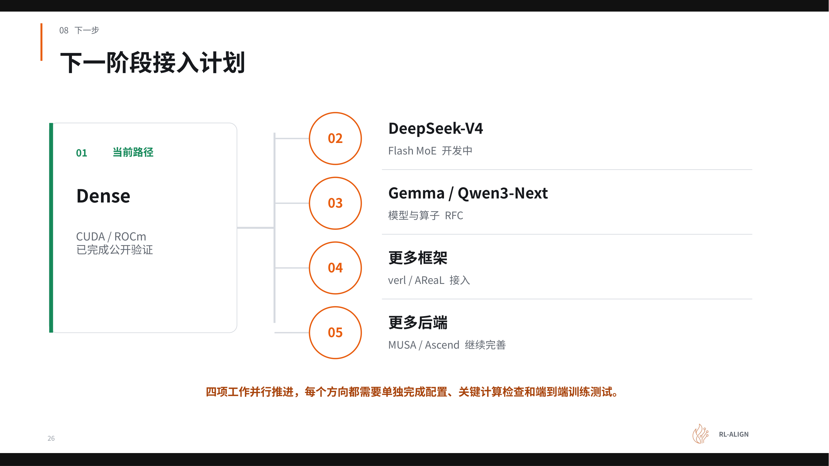Figure: Next-phase integration plan. Item 01 on the left is the currently verified path; items 02–05 on the right are the four parallel evolution directions. Source: Presentation slides, page 26.

The meaning and progress of each branch in the figure:

Branch 02 — DeepSeek-V4 (MoE architecture, the model planned for integration in the next phase). Highest priority; the core team is developing Flash MoE operators. The key difference between MoE and Dense is that each token activates only a subset of experts, and the routing decision itself may introduce nondeterminism. The routing logic must be synchronized between the Rollout and Training sides to maintain LogP consistency.

Branch 03 — Gemma (one of the models planned for integration in the next phase) and more models. The project has submitted an RFC (Request for Comments), and community contributors have started claiming adaptation work, with priority given to completing it on both CUDA and ROCm platforms.

Branch 04 — verl / AReaL (asynchronous reinforcement learning framework) and more frameworks. The current version uses vime as the scheduling framework. Integrating more frameworks means RL-Kernel needs to position itself as a pluggable computation layer, decoupled from the upper-level scheduling logic.

Branch 05 — MUSA (Moore Threads' hardware backend computing platform) / Ascend and more hardware backends. Each backend requires independent verification of numerical consistency—exactly the complete verification pipeline that v0.1.0 has already established on CUDA/ROCm.

Summary

v0.1.0 demonstrated the engineering feasibility of "zero train–inference LogP discrepancy" in the simplest Dense single-node scenario. However, from Dense to MoE, from single-node to multi-node, and from a single framework to ecosystem compatibility, each step introduces new sources of nondeterminism. Train–inference consistency is not a feature delivered once and for all; rather, it is a continuous engineering effort that must evolve in tandem with model architectures, hardware backends, and scheduling frameworks.

---

Conclusion

1. Root cause of discrepancy is clear: The LogP discrepancy in large-model RL post-training originates from differences in GPU floating-point reduction order and precision conversion positions, not from model parameters or input data. This discrepancy is amplified by the importance ratio, prematurely triggers gradient clipping, and seriously threatens training stability.

2. Diagnosis must be layered: Before addressing the consistency problem, the five baseline prerequisite conditions—weight version, input boundaries, positional information, logical state, and stochastic conditions—must be strictly aligned first; otherwise, the diagnostic direction will go astray.

3. Full coverage of five reduction classes: RL-Kernel v0.1.0 established numerical contracts to impose unified constraints on the tiling strategy, merge order, and precision boundaries of five classes of critical reduction operators: RMSNorm, Attention, GEMM/SwiGLU, Linear LogP, and Collectives.

4. Zero discrepancy on two platforms: On the Qwen3-8B Dense model, RL-Kernel achieved 0 mismatch over 200 RL steps on both CUDA (8×H100, TP4/CP2, Global Batch 128) and ROCm (8×MI300X, TP4/CP2, Global Batch 8) platforms.

5. No significant performance sacrifice: Through optimizations such as reusing packed weights, eliminating redundant LM-head GEMM, and using fixed-tree communication topologies, the overhead introduced by alignment constraints was effectively offset, and end-to-end performance remained essentially on par with the native path.

6. Reusable verification methodology: The closed-loop process of fixed replay to strip sampling stochasticity → layer-by-layer comparison to locate the first divergence point → regression to online training after the fix constitutes a standardized numerical consistency diagnostic methodology.

7. Clear evolution direction: The project's next steps will extend to MoE architecture (DeepSeek-V4), more models (Gemma), more frameworks (verl, AReaL), and more domestic hardware backends (MUSA, Ascend).

Applicability limitations:

• All performance and 0 mismatch conclusions have only been verified on the Qwen3-8B Dense model, specific hardware, and specific parallelism configurations, and cannot be directly generalized.
• Whether eliminating LogP mismatch leads to stable improvement in training benefits still requires further verification over longer training horizons and with multiple seeds.
• The CUDA and ROCm experiments used different Global Batch configurations; the absolute runtimes on the two hardware setups cannot be directly compared across platforms.
• The presentation materials did not provide specific throughput numbers or per-item latency breakdowns; "performance on par" is a qualitative conclusion.