Low-Bit Quantization in Practice with vLLM: Core Mechanisms and Architectural Optimizations of AutoRound

Source video: Bilibili BV1etjE69Efx · Slides: Companion materials

Starting from the tension between clipping and rounding, this article dissects SignSGD-based joint optimization and CFG parallel acceleration.

---

Target audience: Backend and AI systems engineers familiar with large-model inference deployment who want a deeper understanding of the underlying quantization mechanisms and vLLM integration principles.

Prerequisites: Basic understanding of floating-point-to-integer mapping; familiarity with Transformer architecture fundamentals and GPU memory usage breakdown; working knowledge of backpropagation in deep learning.

Reading objectives

1. Understand the adversarial relationship between rounding error and clipping error during quantization.
2. Master the block-wise joint optimization principle of AutoRound based on SignSGD.
3. Clarify the differences between QDQ fake quantization in the tuning stage and real INT4 inference.
4. Learn how memory footprint reduction unlocks architecture-level acceleration such as CFG parallelism.

---

1. The Engineering Contradiction: The Imbalance Between Compute and Memory Bandwidth

Question this section answers: In inference deployment of Large Language Models (LLMs) and Vision-Language Models (VLMs), what is the real bottleneck? Why is low-bit quantization no longer an optional optimization but a physical prerequisite for making a service run at all?

The Zero-Sum Game Inside GPU Memory

GPU memory is a fixed-size pie, and an inference service must divide it between two types of expenditure:

Item	Description	Relationship to Quantization
Model weights	Parameters of all layers reside in memory	Halving bit-width → halving footprint
KV Cache	Cached Key/Value attention states for each concurrent request	Smaller weights → more remaining space

The relationship is straightforward: the fatter the weights, the less room is left for the KV Cache, and the fewer requests can be handled concurrently. When the weights swell close to the memory ceiling, even a single request cannot be launched—the problem escalates from "runs slowly" to "cannot run at all."

Prefill vs. Decode: Switching Between Two Bottlenecks

A single inference request consists of two phases, each facing a fundamentally different hardware bottleneck:

• Prefill phase — processes the entire input token sequence at once; matrix operations are dense; this is a compute-bound scenario with relatively high GPU utilization.
• Decode (token-by-token generation) phase — produces only one token per step; reads all weights each time but performs only a small number of multiply-add operations; this is a memory-bandwidth-bound scenario where the GPU spends most of its time waiting for data transfers.

As concurrent requests grow, the Decode phase also gradually shifts toward the compute-bound regime—bandwidth and compute become tight simultaneously.

The figure below illustrates, from a hardware perspective, the quantitative relationship between bit-width and computational efficiency, helping explain why lowering the bit-width relieves pressure along both the compute and bandwidth dimensions at the same time.

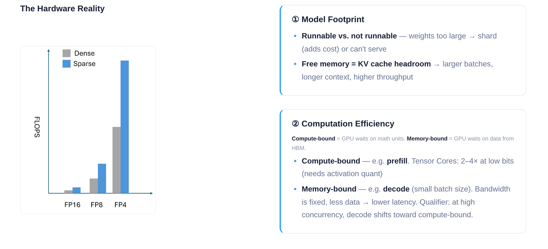Figure: Slide 7 of the presentation. The bar chart on the left compares the compute throughput scaling trend across FP16, FP8, and FP4 under Dense and Sparse execution; the two text boxes on the right explain, respectively, how model size affects "whether it can run" and KV Cache headroom, and the bottleneck difference between Prefill (compute-bound) and Decode (memory-bound).

From the bar chart on the left: as bit-width drops from FP16 to FP8 and then to FP4, available FLOPS increases multiplicatively—the same GPU can complete far more operations per unit time. Layering Sparse execution on top amplifies the gain further. The right side highlights two key evaluation dimensions: model size determines "whether it can run," and computational efficiency determines "how fast it runs."

An Intuitive Scenario

Suppose a GPU has 24 GB of memory. A 7B-parameter model stored in FP16 occupies roughly 14 GB of weights, leaving 10 GB for the KV Cache and runtime overhead. Switching to 4-bit quantization shrinks the weights to approximately 3.5 GB, expanding the available KV Cache space to over 20 GB—concurrency can potentially improve by several times. Meanwhile, the number of bytes that must be read from memory at each Decode step is also reduced to one quarter of the original, alleviating the bandwidth bottleneck accordingly.

Summary

Lowering the bit-width solves problems on two levels simultaneously: on the space level, it frees GPU memory for the KV Cache to boost concurrency; on the bandwidth level, it reduces the data transfer volume per step to accelerate Decode. This is the fundamental reason low-bit quantization has shifted from an "optional optimization" to a "deployment necessity."

However, quantization is not cost-free. Mapping continuous floating-point values to discrete integer levels inevitably introduces rounding error and clipping error, both governed by a shared scale factor and mutually constraining each other. How to find the optimal balance point within this tension is the core problem to be unpacked next.

---

2. The Core Bottleneck: The Zero-Sum Game Between Rounding and Clipping

Question this section answers: Why does naïve Post-Training Quantization (PTQ) struggle to maintain model accuracy at very low bit-widths (e.g., 4-bit)?

The Essence of Quantization: A Lossy Mapping from High to Low Precision

Quantization maps floating-point numbers to a smaller set of discrete integer levels and requires two key steps:

1. Scaling: Compute the ratio between the tensor's maximum absolute value and the largest representable value at the target precision to obtain the scale factor.
2. Rounding: Snap the scaled floating-point value to the nearest integer grid point.

Both steps introduce error. The crux is that the errors are not of a single kind but of three kinds—they share the same control knob and work against each other.

Three Types of Error and Their Trade-Offs

The figure below visualizes the three sources of error and the trade-off among them—an essential prerequisite for understanding the optimization designs that follow.

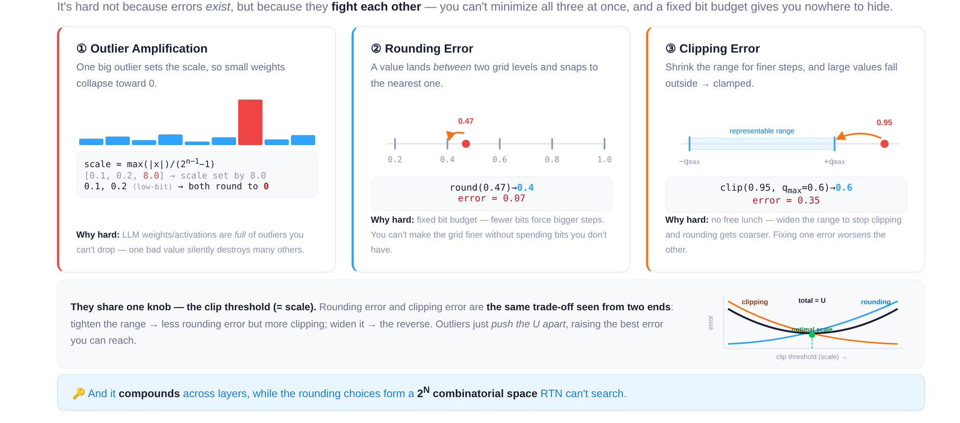Figure: Illustration of three types of quantization error—outlier amplification, rounding error, and clipping error—along with the U-shaped trade-off curve controlled by the clipping threshold. Source: Slide 10 of the presentation.

The figure contains four panels, corresponding to the three error types and one trade-off curve:

Panel ①: Outlier Amplification. The bar chart shows a set of weights mostly concentrated around 0.1–0.2, with a single outlier at 8.0. Because the scale is determined by the tensor's maximum value, the presence of 8.0 forces the scale to be very large. After dividing by the scale and rounding, all small values collapse to 0, and the information they carried is completely lost.

Panel ②: Rounding Error. On the number line, the true value 0.47 falls between two representable grid points, 0.4 and 0.5. Round-to-Nearest (RTN) snaps it to 0.4, producing an error of 0.07. The wider the grid spacing, the higher the expected rounding error.

Panel ③: Clipping Error. When the quantization range is deliberately narrowed to obtain denser grid points, values outside the range are forcibly clamped. In the figure, 0.95 is clipped to 0.6, producing an error of 0.35.

Bottom panel: U-shaped trade-off curve. The horizontal axis is the clip threshold and the vertical axis is error magnitude:

Clip Threshold ↑	Clipping Error	Rounding Error
Increases	↓ More values fall within range	↑ Grid spacing widens
Decreases	↑ More values are clamped	↓ Grid becomes denser

The two error curves intersect to form a U-shaped valley—the theoretically optimal trade-off point. But this "optimum" holds only for a single layer; errors accumulate across layers, and the combinatorial search space grows exponentially (\(2^N\)) with the number of rounding decisions to be made. RTN is powerless against this.

Minimal Example: The Irreconcilable Conflict at 4-Bit

Consider a simplified weight vector [0.1, 0.2, 0.15, 8.0] to be quantized to 4-bit unsigned integers (representable range 0–15).

Strategy A: No clipping; retain the outlier. scale = 8.0 / 15 ≈ 0.533. After quantization, 0.1, 0.2, and 0.15 all round to 0; dequantized result: [0, 0, 0, 8.0]—information from the first three weights is entirely lost.

Strategy B: Clip the outlier to 0.6. scale = 0.6 / 15 = 0.04. Small values now gain discriminability (dequantized results ≈ [0.12, 0.20, 0.16]), but 8.0 is clamped to 0.6 with an error as large as 7.4.

Neither strategy can preserve both large and small values simultaneously. RTN can only perform nearest rounding given a fixed scale; it cannot search the per-element decision space of "round up or round down" globally.

Summary

The root cause of quantization error is not the mere existence of error, but the fact that three types of error share a single clip threshold as the control variable, forming a zero-sum constraint that cannot be simultaneously minimized. At 8-bit quantization, grid points are dense enough for this tension to remain tolerable; when the bit-width drops to 4-bit or below, grid spacing widens sharply, and the tug-of-war between outliers and small values becomes irreconcilable. This is precisely why learnable rounding directions and adaptive clipping ranges must be introduced in very-low-bit scenarios.

---

3. Core Design: Block-Wise Joint Optimization Based on SignSGD

Question this section answers: How does AutoRound (a post-training quantization algorithm) incorporate both rounding error and clipping error into a single optimization loop under a limited compute budget?

The previous section revealed the core of the tension: GPTQ compensates rounding error at the individual Linear layer level, and AWQ protects critical weights based on activation distributions—both operate only at layer granularity and cannot simultaneously adjust rounding directions and clipping ranges. AutoRound's solution is to model quantization as a differentiable discrete optimization problem, jointly learning the optimal rounding offsets and clipping boundaries at the Transformer Decoder Block granularity.

Optimization Variables

AutoRound introduces a continuous rounding offset \(v\) for each weight and also treats the clipping boundaries \(\text{min}\) and \(\text{max}\) as learnable parameters; all three are jointly tuned. The table on the left side of the figure below lists the shapes and initial values of these three variable types, and the right side shows the block-wise iterative algorithm flow.

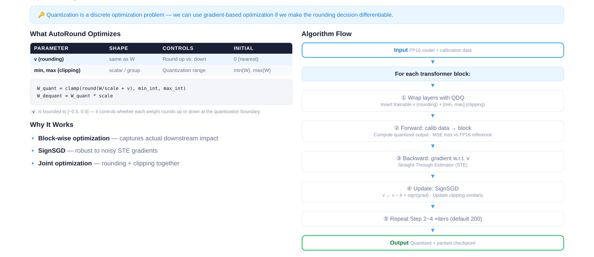Figure: Left — table of three learnable parameter types (v, min, max) with their shapes and initial values; right — block-wise iterative algorithm flow. Source: Slide 11 of the presentation.

The semantics of the three parameter types are as follows:

Parameter	Shape	Controls	Initial Value
\(v\)	Same shape as the weight tensor	Whether each element rounds up or down	\(0\) (default nearest rounding)
\(\text{min}\)	One scalar per group	Lower clipping bound	Group-wise minimum from calibration data
\(\text{max}\)	One scalar per group	Upper clipping bound	Group-wise maximum from calibration data

\(v\) is constrained to the interval \([-0.5,\; 0.5]\). When \(v_i > 0\), the corresponding weight tends to round up; when \(v_i < 0\), it tends to round down. This transforms the originally discontinuous "round-up or round-down" decision into a search in continuous space.

Why Block-Wise Optimization

AutoRound does not calibrate at the individual Linear layer but operates at the Transformer Decoder Block level. A single Block contains multiple sub-layers such as Attention and MLP; quantization error propagates and accumulates across them. Block-wise optimization allows error signals from downstream sub-layers to back-propagate to upstream weights, thereby capturing inter-layer coupling effects.

Compared with global optimization, the block-wise approach has a memory footprint proportional only to the parameter count of a single Block. For large models with dozens of Decoder Blocks, processing blocks sequentially enables single-GPU quantization.

Algorithm Flow

Corresponding to the flow chart on the right side of the figure, the optimization steps for each Block are:

1. Wrap: Replace the Linear layers in the current Block with their QDQ (Quantize-Dequantize, fake quantization) counterparts, inserting the three groups of learnable parameters \(v\), \(\text{min}\), and \(\text{max}\).
2. BF16 reference forward: Run one forward pass on the calibration data with the original BF16 weights and collect the Block's output as the reference.
3. QDQ forward: Run another forward pass with the fake-quantized weights to obtain the quantized output.
4. Backward: Compute the MSE loss between the BF16 reference output and the QDQ output; back-propagate gradients.
5. SignSGD update: Update \(v\), \(\text{min}\), and \(\text{max}\) using SignSGD.
6. Iterate: Repeat steps 3–5 for approximately 200 rounds by default (an empirical hyperparameter).
7. Once the current Block's optimization is complete, freeze its parameters and pass the quantized output to the next Block.

SignSGD: Why Use Only the Sign of the Gradient

The quantization function is essentially a step function and is non-differentiable. In practice, the Straight-Through Estimator (STE) is used to approximate the gradient. However, the magnitude of the STE gradient is highly noisy, whereas its sign (positive or negative) is relatively stable—sufficient to indicate "whether the current \(v_i\) should increase or decrease."

The update rule of SignSGD (Sign Stochastic Gradient Descent) is:

\[\Delta w = \alpha \cdot \mathrm{sign}(grad_w L)\]

where \(\alpha\) is a fixed learning rate and \(grad_w L\) is the gradient of the loss with respect to the parameter. The update magnitude is independent of the gradient magnitude; each step makes a uniform \(\pm\alpha\) move. For \(v\), whose search space spans only \([-0.5, 0.5]\), uniform-step progression is a natural fit for this bounded discrete problem.

Minimal State-Evolution Example

Suppose a certain weight has a floating-point value of \(3.3\):

• Default nearest rounding: \(v=0\), quantized value is \(3\), rounding error is \(0.3\).
• After several rounds of SignSGD: The optimizer discovers that increasing \(v\) (rounding up to \(4\)) raises the local error to \(0.7\), yet the MSE of the entire Block's output actually decreases—because downstream layers are highly sensitive to this weight, and \(4\) yields smaller propagation error than \(3\).
• Simultaneously, \(\text{min}\)/\(\text{max}\) are also being adjusted, potentially moderately narrowing the clipping range to reduce the stretching effect of outliers on the scale.

All three work in concert, driving the Block output MSE to converge to the joint optimum during iteration.

Summary and Boundaries

By unifying rounding offsets and clipping boundaries as learnable parameters and solving iteratively with SignSGD at the Decoder Block granularity, AutoRound breaks the static trade-off between rounding and clipping at relatively low memory and compute cost. Its boundary lies in the fact that the default 200 iterations is an empirical hyperparameter; in very-low-bit scenarios (e.g., 2-bit or MXFP4), the adaptive mixed-precision and lightweight stabilization strategies introduced by SignRound V2 are needed to further narrow the accuracy gap (SignRound V2 was published on arXiv in 2025).

Once the algorithm design is mathematically sound, the engineering question becomes: how does the QDQ fake quantization mechanism enable gradient back-propagation during tuning without incurring the overhead of real low-precision arithmetic?

---

4. Data Structures and Execution: QDQ Fake Quantization vs. Real Inference

Core question of this section: For the same quantized model, at what precision do tensors actually participate in computation during offline tuning versus online inference? Why must the two paths be designed separately?

Comparing the Two Data Paths

The figure below places the tuning-stage and inference-stage computation flows side by side, clearly revealing the essential difference between "fake quantization" and "real quantization."

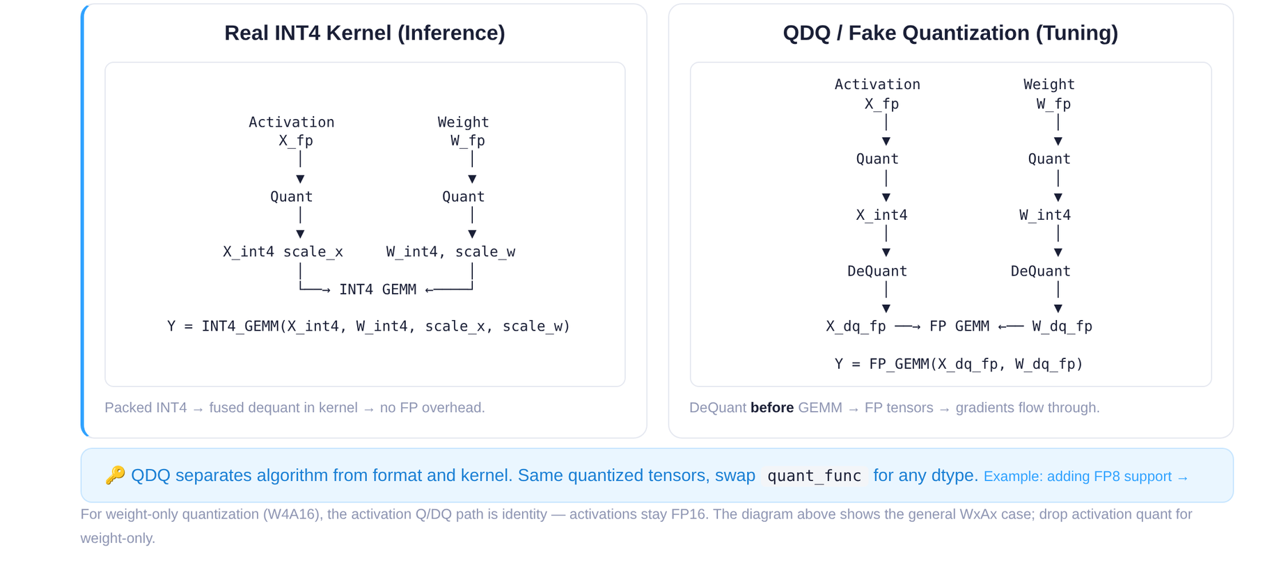Figure: Left — Real INT4 Kernel path during inference; right — QDQ fake quantization path during tuning. Source: Slide 14 of the presentation.

Dimension	Real INT4 Kernel (Inference)	QDQ / Fake Quantization (Tuning)
Core operation	Fused dequantization inside the kernel; directly executes INT4 GEMM	Quantize to INT4, then dequantize back to FP, then execute FP GEMM
Output precision	Low-bit result returns to FP after fused dequantization	Remains in FP throughout
Gradient retention	No (pure forward inference)	Yes (gradients can be back-propagated on FP tensors)
Performance objective	Eliminate floating-point overhead; maximize throughput	Speed is not the goal; fidelity of error simulation is

Left path (Inference): FP weights are quantized to INT4 before entering the kernel. The kernel internally performs matrix multiplication with integer instructions and completes fused dequantization upon write-back. No extra floating-point intermediate tensors are produced in the entire process.

Right path (Tuning): The FP tensor is likewise quantized to INT4, but then immediately dequantized back to FP space; subsequent operations are standard FP GEMM. This "compress then decompress" step is QDQ (Quantize-Dequantize, fake quantization)—its purpose is not acceleration, but to inject a segment of "quantization noise" into the FP computation graph so that the downstream MSE loss can perceive the precision deviation introduced by low bit-width.

Why the Tuning Stage Must Take the QDQ Path

The causal chain can be described in three steps:

1. Gradient back-propagation requires floating-point tensors. The SignSGD optimizer described in the previous section needs to perform gradient updates on \(v\), \(\text{min}\), and \(\text{max}\). If the tensor has already been truncated to integers, gradients cannot flow back through the computation graph.
2. Error simulation requires the real quantization function. The Quantize step in QDQ invokes the same mapping as the final inference kernel, so the simulated error is "real."
3. Data-type decoupling provides flexibility. When a new data type needs to be supported (e.g., FP8 or MXFP4), one only needs to implement a tensor-level QDQ function and register it with AutoRound to evaluate the new schema's impact on accuracy—without waiting for the corresponding hardware kernel to be ready.

Compatibility with Block-by-Block Loading: Single-GPU Quantization Even for Very Large Models

The QDQ path is naturally compatible with AutoRound's per-Decoder-Block loading strategy. During quantization, the main process loads the current Block from CPU DRAM to GPU VRAM, inserts QDQ nodes before and after each Linear layer in that Block, iteratively optimizes them, offloads the results back to DRAM, and then loads the next Block. Because QDQ always runs as FP GEMM and does not depend on specific low-bit hardware instructions, any GPU supporting FP arithmetic can execute it. Even for models with 600B parameters, the memory requirement is only the size of a single Block plus a small activation buffer.

Minimal State Evolution

Suppose an element of a layer's weight has an original value of w = 0.37 (BF16), with scale = 0.05 and zero = 8:

Step	Operation	Value
① Quantize	Map to INT4 range [0, 15]	q = round(0.37/0.05) + 8 = 15 (clamp)
② Dequantize	Map back to FP	w' = (15 − 8) × 0.05 = 0.35
③ FP GEMM	Use w' = 0.35 in matrix multiplication	Introduces quantization error Δ = 0.02
④ Loss & Grad	MSE loss perceives Δ; gradient back-propagates to the scale parameter	Scale is fine-tuned

During inference, steps ② and ③ are fused into the INT4 kernel, eliminating the FP intermediate value.

Boundaries and Limitations

• For weight-only quantization (e.g., W4A16), activations are not quantized; QDQ acts only on weight tensors.
• Tiny numerical differences may exist between the precision loss simulated by QDQ and the actual kernel behavior (e.g., differences in rounding mode); the presentation materials do not provide per-layer deviation data between the two.
• When the hardware kernel for a target data type is not yet available, QDQ is the only means of precision evaluation; once the kernel becomes available, deployment should always switch to the real kernel for actual speedup.

After offline quantization is complete and the checkpoint is exported, the next question is: how is this low-bit weight file automatically recognized by the vLLM inference framework and connected to the underlying accelerated operators?

---

5. System Overview: Quantization Interception and Dispatch in the vLLM Architecture

Question this section answers: What path does an AutoRound-produced checkpoint follow before it is automatically recognized inside vLLM (an open-source LLM serving framework) and ultimately dispatched to highly optimized low-level operators such as Marlin?

Offline Quantization: From Full Precision to a Deployable Checkpoint

The deployment starting point is an offline quantization process, not a dynamic conversion at inference time. The figure below shows the complete workflow from full-precision weights to online serving.

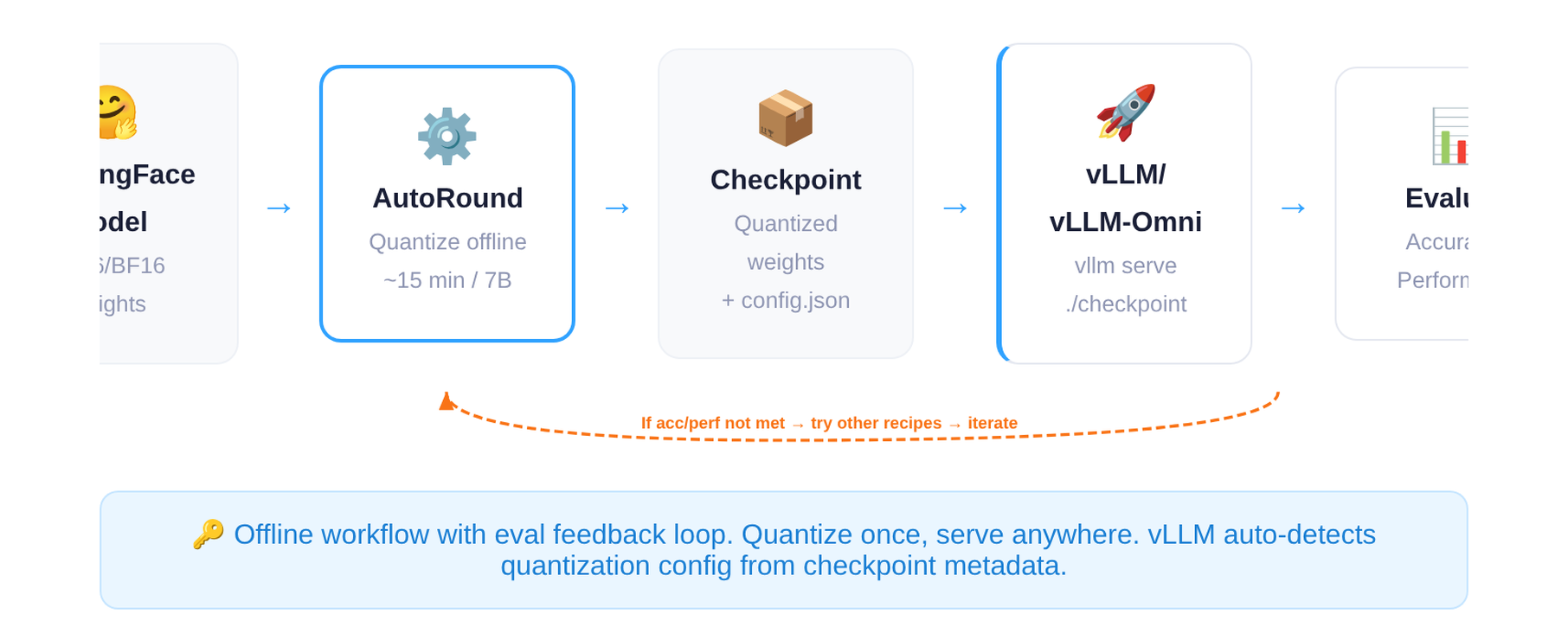Figure: AutoRound deployment workflow—from HuggingFace full-precision weights to vLLM online serving. Source: Slide 20 of the presentation.

Key nodes in the end-to-end workflow:

Stage	Input	Output	Notes
Offline quantization	HuggingFace model (FP16/BF16)	Checkpoint (quantized weights + config.json)	~15 minutes for a 7B model
Service loading	Checkpoint directory	vLLM / vLLM-Omni online engine	vLLM reads config.json to auto-detect the quantization format
Evaluation feedback	Accuracy and performance metrics	Decision: deploy or iterate	If metrics fall short of expectations, re-quantize with a different scheme

Note: The 15-minute quantization time refers specifically to a 7B-scale model; larger models take correspondingly longer.

The core artifact is a device-agnostic checkpoint. The quantized weight files can be shared across Intel XPU, CUDA GPU, HPU, and even CPU, as long as the target device has a corresponding inference kernel available.

Inside vLLM: From Layer Dispatch to Quantization Operators

Once the checkpoint is loaded, the low-bit weights do not simply participate in a standard forward as ordinary tensors. During model initialization, vLLM inspects the quantization metadata declared in config.json and replaces standard linear layers with dedicated quantization linear layers (Quantization Layers); at runtime, execution automatically follows the optimized path.

The figure below shows vLLM's architectural layering and the call stack of a quantized Linear, illustrating where "layer replacement" fits within the overall system.

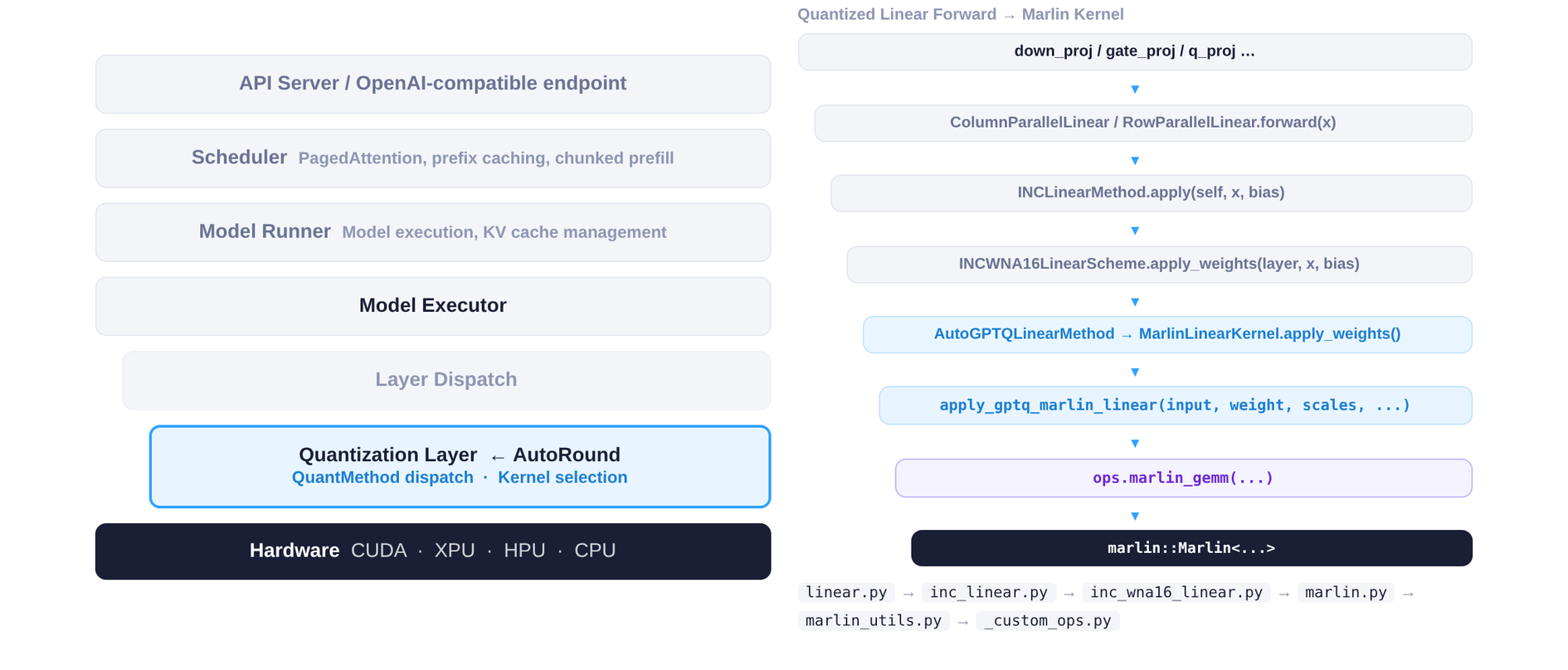Figure: Left — vLLM architectural layering; right — call stack from quantized Linear Forward to Marlin Kernel. Source: Slide 8 of the presentation.

Left — Architectural layering (top-down): API Server receives requests → Scheduler batches and schedules → Model Runner drives forward computation → Layer Dispatch traverses each layer and determines the execution path → Quantization Layer (AutoRound) intercepts the standard linear operation here → Hardware executes the actual computation. AutoRound is embedded between Layer Dispatch and Hardware; the upper scheduling layers need not be aware of whether weights are quantized, achieving decoupling of scheduling and operators.

Right — Call stack: Starting from the PyTorch-level linear projection (e.g., QKV Projection), the call passes through vLLM's quantization dispatch logic and ultimately lands on the C++-level Marlin GEMM operator—a matrix-multiplication kernel highly optimized for low-bit weights. The Python layer is responsible only for "selecting the path"; the compute-intensive portion is handled entirely by the C++ layer.

Minimal Example: The Lifecycle of a Single Quantized Inference Request

Using an INT4-quantized 7B model as an example:

1. Offline: AutoRound quantizes the BF16 weights; config.json is tagged with "quant_method": "auto_round".
2. Loading: At startup, vLLM scans config.json, identifies the quantization scheme, and replaces all applicable nn.Linear modules with quantization linear layers.
3. Inference: Request arrives → Scheduler batches it → When the Attention QKV projection is reached, Layer Dispatch routes the call to the Quantization Layer → The Marlin Kernel executes INT4 × FP16 matrix multiplication → The result is returned to the upper layers.
4. Evaluation: If accuracy or throughput falls short of expectations, return to the offline stage, adjust the recipe, and re-iterate.

Summary and Boundaries

vLLM adopts a "metadata-driven layer replacement" strategy: the offline stage solidifies quantization decisions into config.json, and the online stage lets the framework automatically perform layer replacement and kernel dispatch. Note: if the quantization fields in config.json are missing or malformed, vLLM falls back to the standard-precision path; layer replacement occurs at model-loading time rather than at runtime, so switching schemes requires reloading the model.

With system integration in place, the benefits of quantization extend beyond mere memory savings—more importantly, the freed memory can unlock entirely new compute-architectural optimizations.

---

6. Optimization Principles and Performance: Memory Reduction Unlocks CFG Parallelism

Question this section answers: Beyond "the model is smaller and fits on fewer cards," how can quantization deliver multiplicative inference speedups at the architectural level?

Background and Bottleneck: The Resource Dilemma of FLUX Under BF16

The Transformer portion of FLUX (a diffusion model) occupies approximately 23 GB of GPU memory at BF16 precision. The Intel XPU B60 has 24 GB of per-card memory—even without loading the VAE, text encoder, or any other components, a single card can barely hold the Transformer itself. Without CPU offloading, at least 4-way tensor parallelism (Tensor Parallel, TP = 4) is required to launch inference.

TP = 4 incurs two costs: first, each All-Reduce introduces cross-card communication latency, and the communication fraction grows with the number of Transformer layers; second, each card must maintain communication buffers and intermediate activations in addition to its model shard, reducing effective utilization.

In diffusion models, CFG (Classifier-Free Guidance) requires two forward passes on the same noisy input—one conditional branch and one unconditional branch—whose results are then combined via weighted blending. Under the BF16 + TP = 4 configuration, the memory of all four cards is already consumed by the model, so the two CFG branches can only be executed serially, directly doubling latency.

The Key Turning Point: W4A16 Compresses 23 GB Down to 7 GB

After applying W4A16 (4-bit weights, 16-bit activations) AutoRound quantization to the FLUX Transformer, the weight memory footprint drops from 23 GB to approximately 7 GB, roughly consistent with the theoretical 4-bit / 16-bit ≈ 1/4 ratio (the extra overhead comes from scale, zero-point, and other metadata). A 7 GB model fits on a single 24 GB B60 card—TP = 1 is sufficient. If the machine has 4 cards, each card has roughly 17 GB of free memory, creating room for parallel strategies.

Architecture-Level Acceleration: CFG Parallelism

The idea behind CFG Parallel is: since memory is now sufficient, place the conditional and unconditional branches on different cards and execute them simultaneously. Taking TP = 2, CFG = 2 as an example:

1. Card 0 + Card 1 compute the conditional branch with TP = 2;
2. Card 2 + Card 3 compute the unconditional branch with TP = 2 at the same time;
3. After both branches complete, merge the guidance results and proceed to the next denoising step.

Compared with the serial path of BF16 TP = 4, CFG = 1—where all four cards first compute branch A and then branch B—CFG parallelism folds two serial forward passes into a single parallel forward pass.

Measured Results

The figure below presents the memory and latency comparison across different configurations—key evidence for the engineering value of quantization.

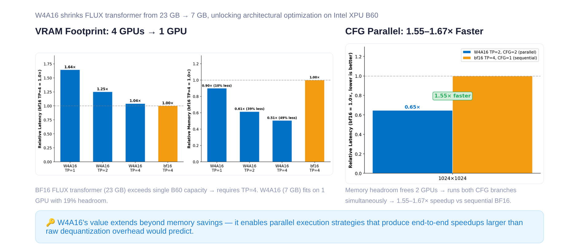Figure: Slide 25 of the presentation. The bar chart on the left shows the memory and latency ratios of W4A16 under various TP configurations relative to the BF16 TP = 4 baseline; the right side shows the speedup factor of CFG parallelism at 1024×1024 resolution.

Key data from the figure:

Configuration	Relative Memory	Relative Latency	Notes
BF16, TP = 4, CFG = 1	1.00× (baseline)	1.00× (baseline)	4-card serial CFG
W4A16, TP = 1	~0.51×	—	Single-card operation
W4A16, TP = 2, CFG = 2	—	~0.61×–0.65×	Both branches in parallel

Under 1024×1024 resolution on Intel XPU B60 hardware, W4A16 TP = 2 + CFG Parallel achieves a 1.55–1.67× end-to-end speedup relative to BF16 TP = 4 with serial CFG. The speedup can be decomposed into two parts: reducing TP from 4 to 2 cuts communication overhead; executing two CFG branches in parallel approximately halves the forward latency of the denoising loop.

Boundary Conditions

1. The numbers above are strictly tied to the Intel XPU B60 (24 GB memory); gains will differ on hardware with different memory capacities and interconnect bandwidths.
2. Only 1024×1024 resolution results are shown; at higher resolutions, activation memory grows and parallel headroom shrinks, potentially reducing the speedup ratio.
3. CFG parallelism is applicable only to diffusion model inference scenarios that require multi-branch guidance; it cannot be directly transferred to the Decode phase of autoregressive LLMs.
4. The entire pipeline's validity presupposes that generation quality after W4A16 quantization remains acceptable—this is exactly what the next section examines.

---

7. Edge Cases: Consistency of Video Generation Models

Question this section answers: When diffusion model weights are compressed from BF16 to 4-bit (W4A16), does the spatiotemporal consistency of generated videos exhibit perceptible degradation?

This question is critical because inter-frame subject consistency and background consistency are extremely sensitive to quantization noise—subtle weight perturbations can be amplified frame by frame along the temporal axis, ultimately leading to flickering, deformation, or even structural collapse.

Objective Metric Comparison

The figure below compares multi-dimensional evaluation scores of the Wan2.2 series models on T2V (Text-to-Video) and I2V (Image-to-Video) tasks, used to determine whether quantization causes structural degradation.

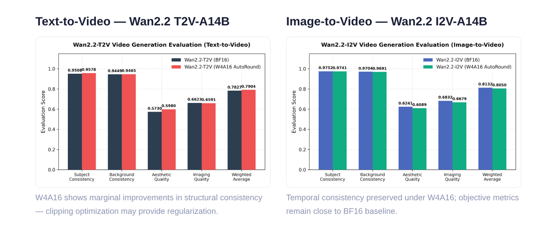Figure: Five objective metrics comparing Wan2.2 T2V-A14B and I2V-A14B under BF16 and W4A16 precision. Source: Slide 24 of the presentation.

The key numbers are organized below (bolded entries indicate that the quantized score exceeds the BF16 baseline):

Dimension	T2V BF16	T2V W4A16	I2V BF16	I2V W4A16
Subject Consistency	0.9508	0.9578	0.9752	0.9741
Background Consistency	0.9449	0.9465	0.9704	0.9691
Aesthetic Quality	0.5730	0.5980	0.6241	0.6089
Imaging Quality	0.6623	0.6591	0.6832	0.6679
Weighted Average	0.7827	0.7904	0.8132	0.8050

T2V scenario: W4A16's Subject Consistency rises from 0.9508 to 0.9578, and Background Consistency also shows a positive shift of roughly 0.002. The weighted average improves from 0.7827 to 0.7904; the quantized version is marginally better overall. The only slightly declining dimension is Imaging Quality (0.6623 → 0.6591), an absolute difference of merely 0.003.

I2V scenario: All five W4A16 scores are slightly below the BF16 baseline, but the decreases are minimal—the largest gap appears in Aesthetic Quality, at approximately 0.015. The two core temporal-consistency metrics each drop by no more than 0.002, indicating that 4-bit quantization has not introduced degradation that accumulates along the temporal axis.

Why Quantization Did Not Cause Visual Collapse

AutoRound's clipping optimization jointly adjusts the clipping boundaries and rounding strategy for each weight group during calibration: narrowing the clipping boundaries makes the quantization interval more compact, effectively suppressing the contribution of outliers to reconstruction error; joint rounding-direction optimization minimizes the per-block error between each layer's output distribution and the BF16 baseline. Combined, the distributions of feature channels critical to subject contour and background structure are preserved.

For the marginal improvement observed in T2V, a plausible hypothesis is that the clipping optimization, by narrowing the weight range, objectively acts as a form of regularization, attenuating the interference of extreme weight values on generated frames. It should be emphasized that this improvement is small; the presentation materials characterize it as a marginal gain and it should not be taken as a general conclusion that quantization outperforms full precision.

Boundary Conditions

The presentation materials do not disclose the specific size or sampling strategy of the evaluation dataset, nor do they provide corresponding data at lower bit-widths (e.g., W2 or W3). The conclusions above currently apply only to W4A16 precision and the Wan2.2-A14B model scale; performance under smaller models or lower bit-width settings remains to be verified.

---

8. Limitations and Practical Considerations: Native Hardware Support and Configuration Trade-Offs

Question this section answers: In real-world deployments, what is the most common reason a quantized model fails to deliver expected speedups?

The answer boils down to two points: the underlying hardware lacks native kernel support for the target low-bit data type; and the quantization recipe's parameters do not match the business scenario.

The First Gate: What Does the Hardware Support?

Before choosing a quantization scheme, the first thing to confirm is not "which precision is the lowest" but "which low-bit types does the target GPU natively support." Without a mature kernel implementation, the theoretical benefits of quantization remain on paper.

Taking Intel's current and roadmapped hardware as an example:

Hardware Product	Natively Supported Low-Bit Types	Availability
Intel Arc GPU B60 / B70	INT8 (including INT4 inference path)	Released
Intel Gaudi	FP8	Released
CRI GPU (next generation)	MXFP4 / MXFP8	H2 2026

MXFP4 (Microscaling 4-bit Floating Point) is a microscaling 4-bit floating-point format that requires dedicated matrix-computation units at the hardware level to achieve throughput gains.

The causal chain is clear: a user quantizes a model to W4 and deploys it, but if the GPU lacks native INT4 instructions, the kernel will first dequantize INT4 to FP16/BF16 and then execute a general-purpose GEMM—the dequantization itself consumes compute and bandwidth, negating the savings from low-bit storage. The end result is "memory is saved, but speed is unchanged or even worse."

The 1.55–1.67× speedup of the FLUX model on the B60 in the previous section was achieved precisely because the B60 natively supports the INT8/INT4 path. Conversely, deploying an MXFP4-quantized model on existing hardware that does not yet support the format will not yield comparable gains.

The Second Gate: Parameter Trade-Offs in the Quantization Recipe

Once hardware feasibility is confirmed, the quantization scheme and hyperparameters must be selected according to business priorities. AutoRound provides four preset modes; the figure below lists their parameter differences and applicable scenarios.

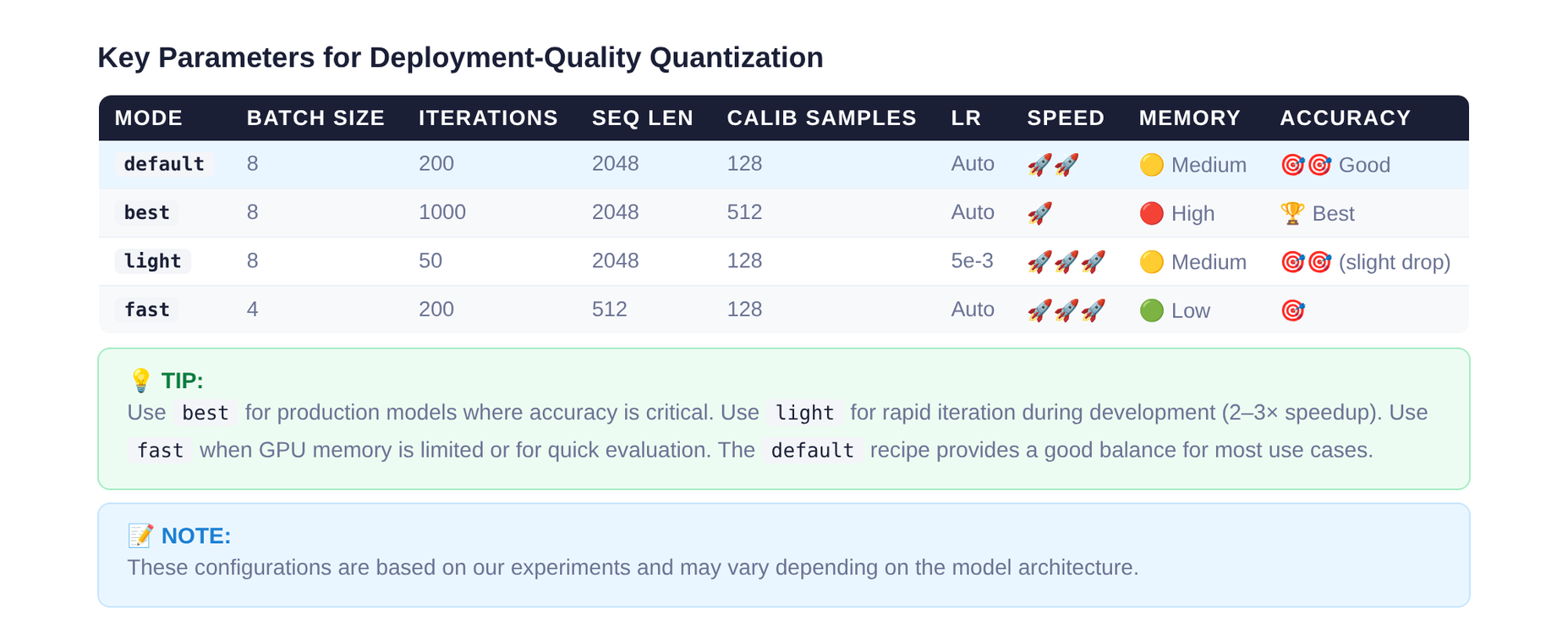Figure: Parameter comparison of AutoRound's four preset modes — default, best, light, and fast. Source: Slide 28 of the presentation.

The key parameter differences are as follows:

Mode	Batch Size	Iterations	Seq Len	Calib Samples	Applicable Scenario
default	8	200	2048	128	Balanced choice for most scenarios
best	8	1000	2048	128	Production-grade accuracy requirements; ~2–3× the time of default
light	8	50	512	128	Rapid validation and development stage
fast	4	200	2048	128	Memory-constrained environments; trades a small amount of accuracy for lower peak memory usage

The impact directions of key variables:

• Iterations: Directly determines the number of SignSGD optimization rounds; best mode increases this to 1000 for higher accuracy, with calibration time growing linearly.
• Seq Len (sequence length): Affects the context range covered by the calibration data; increasing from 512 to 2048 improves quantization quality for long-text scenarios, but memory usage increases accordingly.
• Batch Size: fast mode reduces it from 8 to 4, lowering peak memory usage and making it suitable for consumer-grade GPUs.
• Learning rate: All modes default to 5e-3; the presentation materials do not provide ablation data for different learning rates.

General principles for scheme selection: When memory is the priority (edge deployment, large models on small cards), choose low-bit combinations such as W4A16; when accuracy is the priority (production environments, quality-sensitive tasks), choose W4A16 with a smaller group_size or W8A8/FP8; for long-context or vision-language model scenarios, KV Cache quantization can be layered on top of weight quantization.

---

Conclusion and Limitations

1. Quantization is not a simple numerical compression but a joint game among three types of error: rounding, clipping, and outlier amplification. All three share the clip threshold as a control variable, forming a U-shaped constraint that cannot be simultaneously minimized.

2. AutoRound models quantization as a differentiable optimization problem. By using SignSGD at the Transformer Decoder Block granularity to jointly learn the rounding offset \(v\) and the clipping boundaries \(\text{min}\)/\(\text{max}\), it breaks the static trade-off of traditional PTQ under a limited compute budget.

3. QDQ fake quantization bridges algorithmic exploration and hardware execution. The tuning stage uses QDQ to simulate error while maintaining gradient back-propagation; the inference stage switches to real INT4 kernels to eliminate floating-point overhead. The separation of these two paths enables even very large models (e.g., 600B parameters) to be quantized block by block on a single GPU with limited memory.

4. The engineering value of quantization extends beyond reducing memory footprint. Taking FLUX as an example, W4A16 compresses the Transformer memory from 23 GB to 7 GB; the freed memory is reinvested in CFG parallelism, achieving a 1.55–1.67× end-to-end speedup on the Intel XPU B60 at 1024×1024 resolution.

5. Very-low-bit quantization does not destroy the spatiotemporal consistency of video generation models. In Wan2.2's T2V/I2V tasks, the structural consistency metrics of W4A16 differ from the BF16 baseline by no more than 0.002, and T2V even exhibits a marginal positive shift.

6. Ultimate inference acceleration strictly depends on native hardware data-type support and highly optimized low-level kernels. On hardware lacking the corresponding kernel, quantization can only save storage and cannot improve throughput.

7. Remaining limitations:

8. Performance numbers (e.g., 1.55–1.67× speedup, 15-minute quantization time) are highly dependent on specific hardware and configurations and cannot be directly generalized.
9. Native hardware support for MXFP4/MXFP8 (CRI GPU) is not expected until H2 2026; until then, INT8 and FP8 remain the safest low-bit options on Intel hardware.
10. The presentation materials do not provide systematic accuracy evaluation data at 2-bit and below; AutoRound's performance in that range awaits further validation through SignRound V2.