Joint Audio-Video Generation in Production: Architecture Deep Dive into MiniMax-H3 and vLLM-Omni

Full-Pipeline Optimization — From the 118 GB VRAM Bottleneck to Multi-Task Mixed Scheduling

Source video: Bilibili BV1xmuT6dE1M · Slides: Companion materials

---

When a video generation model begins to simultaneously output frames and stereo audio, the deployment engineer no longer faces a localized issue such as "a single operator is slow." Instead, it is a systemic challenge created by the triple superposition of model size, sequence length, and iteration count. MiniMax-H3 places video frames and native stereo waveforms into the same denoising pipeline using a shared DiT (Diffusion Transformer), achieving strict audio-video synchronization at the algorithmic level. vLLM-Omni, in turn, provides a complete engineering solution at the inference-serving level for this behemoth — from VRAM offloading to step-level scheduling. This article follows a causal chain — "Where is the bottleneck → How is the architecture decomposed → How does data flow → How is VRAM saved → How are kernels stabilized → How is latency compressed → How is deployment landed" — to dissect the core design and engineering trade-offs of this joint generation system.

Target audience: AI systems engineers with a foundation in large-model inference who want to understand multi-modal DiT joint generation mechanisms and production-grade deployment optimization.

Prerequisites:

• Basic concepts of Diffusion Transformers (DiT) — noise scheduling, denoising loop, velocity parameterization
• Basic architecture of the vLLM inference framework — scheduler, Worker, model executor
• Principles of Tensor Parallelism (TP) and CPU VRAM offloading

Reading objectives:

1. Understand the unified architectural design of MiniMax-H3's joint audio-video generation and the systemic overhead it introduces
2. Master vLLM-Omni's VRAM reuse strategy through multi-task routing and shared components
3. Gain insight into inference optimization mechanisms such as DLO, step-level scheduling, and cross-step caching, along with their applicable boundaries

---

1. Unified Architecture and the 118 GB VRAM Wall

Key question for this section: Why does a joint audio-video generation model simultaneously hit both a VRAM peak and an inference latency wall when going into production deployment?

Why Unification Is Necessary

The conventional approach assigns video and audio to two independent generation models for separate processing, then aligns audio-video timing through post-processing. The flaw in this separated path is that the two sampling chains are independent; timing alignment can only "catch up after the fact," resulting in unstable quality.

MiniMax-H3 takes a more aggressive route — using a single 33B-parameter DiT to simultaneously process video frames and native stereo waveforms. The end-to-end pipeline can be summarized in four steps:

Stage	Component	Output
Condition encoding	Qwen3-VL (2B text-vision encoder)	Text and image condition vectors
Sequence packing	Video latent + audio latent + text token concatenation	A mixed sequence containing 58,758 effective tokens
Denoising backbone	Shared 33B DiT × 50 steps	Joint audio-video velocity field
Decoding	Dual-path VAE (Video VAE + Audio VAE)	Synchronized video frames and stereo waveforms

VAE (Variational Autoencoder) is responsible here for latent-space encoding and decoding of video and audio, respectively.

The unified path allows audio and video to share an attention context at every denoising step, guaranteeing temporal alignment by design. However, this also means the computational cost of all modalities is stacked onto the same inference hot path.

The Triple Multiplier on the Hot Path

The diagram below illustrates how three pressure sources on the inference main pipeline amplify overhead stage by stage — the starting point for understanding all subsequent optimization techniques.

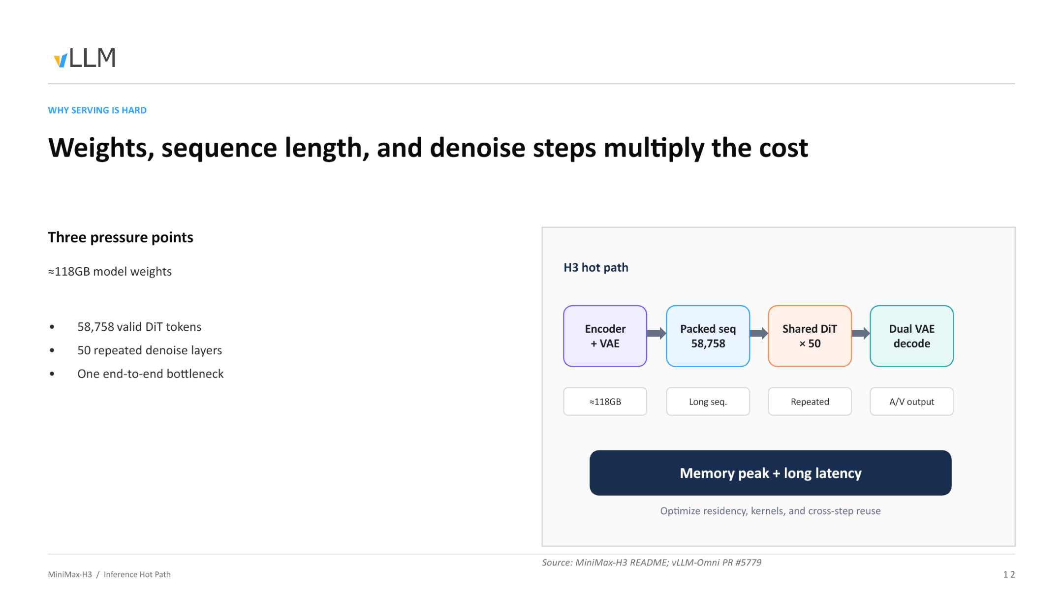Figure: The three major pressure points on the inference hot path and their compounding relationship. Source: presentation slides, page 12.

From left to right, the diagram shows four stages — condition encoding, sequence packing, DiT denoising, and dual VAE decoding — with the primary overhead type annotated below each stage:

1. ≈ 118 GB model weights — the combined total of the encoder (Qwen3-VL, 2B), the shared DiT (33B), and the dual-path VAE decoders. Keeping all of them resident in GPU VRAM alone approaches or exceeds the physical limit of a single card (80 GB A100 / H100).
2. 58,758 effective DiT tokens — the sequence length after concatenating video latents, audio latents, and text tokens. The VRAM and FLOPs for attention computation grow super-linearly with sequence length, making a single forward pass itself extremely expensive.
3. 50-step denoising loop — all layers of the DiT must be executed repeatedly 50 times (one full forward pass per step). The attention computation over 58,758 tokens is not performed once, but 50 times.

The relationship among these three is not simple addition but a multiplier effect — growth in any single dimension proportionally amplifies the burden imposed by the other two.

From Input to OOM: The VRAM Inflation Trajectory of a Single Request

1. Text input — The user submits a video generation prompt; the text token count is on the order of tens to hundreds.
2. Condition encoding — Qwen3-VL encodes the text into condition vectors; initial noise latents for video and audio are sampled. Encoder weights must be loaded.
3. Sequence concatenation — Video latents, audio latents, and text condition vectors are packed into a long sequence of 58,758 tokens; activation VRAM surges accordingly.
4. 50-step denoising — The 33B DiT performs 50 rounds of forward passes over the long sequence; each round requires full model weights to be resident plus intermediate activations. Peak VRAM is reached during this stage.
5. Dual VAE decoding — After denoising completes, audio and video latents are fed into their respective VAE decoders. If DiT weights are still resident in VRAM, the additional decoder weights will trigger OOM.

Step 4 is the absolute bottleneck: it simultaneously requires 118 GB-class weight residency, 58,758-token-class activation caching, and the time overhead of 50 iterations.

Conclusion

The unified DiT solves the audio-video synchronization problem at the algorithmic level, but creates a VRAM wall at the systems level — one formed by the triple superposition of weight size, sequence length, and denoising step count. To push the model into production, each stage must be decoupled at the architectural level, with targeted strategies applied separately for VRAM residency, compute kernels, and cross-step reuse.

Boundary conditions: 58,758 tokens is the effective DiT token count given in the presentation materials; the actual sequence length may vary with input resolution and duration. 118 GB is an approximate value, depending on precision configuration and whether dual-task weights are loaded simultaneously.

Since loading all 118 GB of weights at once is infeasible, how does the system reduce redundant VRAM consumption in multi-task scenarios through architectural design?

---

2. Shared Shell and Multi-Task Dynamic Routing

Key question for this section: When supporting multiple tasks such as text-to-video and reference-video continuation, how can we avoid loading a full model copy for each task type?

Two Tasks, Two DiTs, One Commonality

MiniMax-H3 supports two major categories of video generation tasks, each corresponding to independently trained DiT weights:

• FL2VA (First/Last frame to Video & Audio): Video and audio generation driven by text or first/last frames
• Ref2VA (Reference to Video & Audio): Continuation generation driven by a reference video

If a complete service were launched for each task type, the Text Encoder and dual VAEs would each need to be stored separately. The key structural fact is: FL2VA and Ref2VA have different DiT weights, but their Text Encoder and dual VAEs are identical. This provides the basis for component reuse.

Combined Serving: Load Once, Serve Two Capabilities

Based on this, vLLM-Omni introduces a Combined Serving mode that splits the model into two layers:

Layer	Component	Instance count	Description
Shared shell	Text Encoder, Video VAE, Audio VAE	Singleton, always resident	All tasks reuse the same encoder/decoder weights
Task-specific core	FL2VA DiT or Ref2VA DiT	Activated on demand	In combined mode, both DiTs coexist in VRAM

The diagram below shows the complete pipeline view of Combined Serving, enabling one to trace the full path of a request from entry to result return.

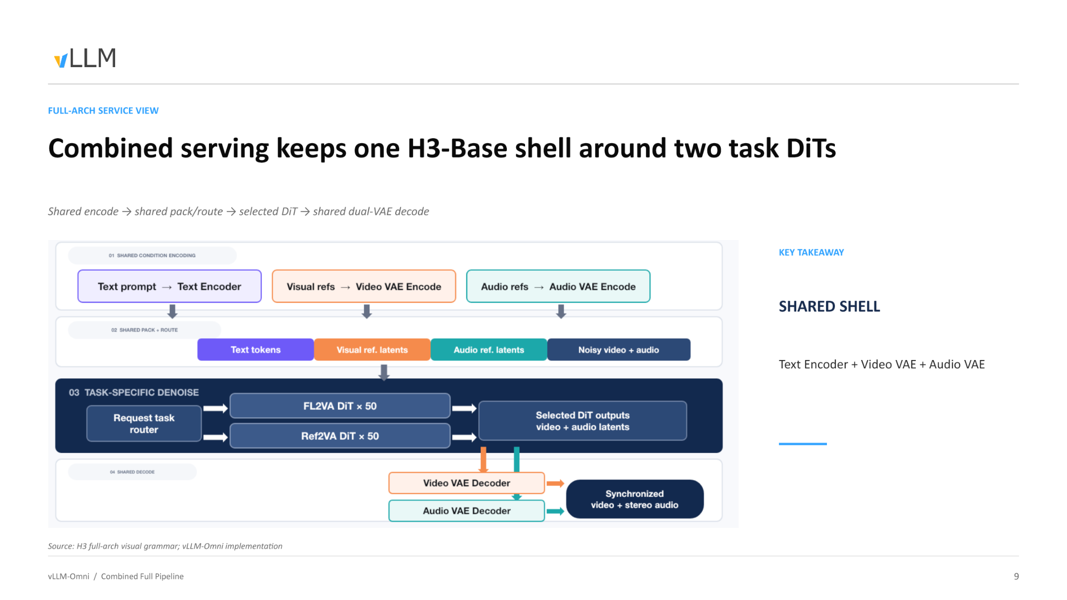Figure: Combined Serving full pipeline. Data enters from the shared encoder on the left, passes through the task router to select a DiT, and is finally decoded by the shared dual VAEs to output synchronized video and stereo audio. Source: presentation slides, page 9.

Following the arrows in the diagram, the causal chain of a single request proceeds as follows:

1. API reception — The client sends a request to a single Video API; the request body carries a task type field (e.g., extra_params.task; exact field name pending verification).
2. Shared encoding — The Text Encoder encodes the text prompt into condition vectors; if reference frames or reference audio are present, the corresponding VAE simultaneously completes latent-space encoding. This step does not differentiate by task type.
3. Dynamic routing — The scheduling layer reads the task identifier in the request: t2va / fl2va routes to the FL2VA DiT, ref2va routes to the Ref2VA DiT.
4. DiT denoising — The selected DiT executes 50 iterative steps, generating a joint video-audio latent-space representation. The other DiT is not invoked during this time.
5. Shared decoding — Denoising results uniformly enter the Video VAE and Audio VAE, outputting synchronized video frames and stereo waveforms.

Launch Modes: On-Demand VRAM Tailoring

Not all scenarios require serving both task types simultaneously. vLLM-Omni uses a --task-type parameter at service startup to determine the loading strategy:

Launch parameter	DiT loaded	Serviceable request types
--task-type fl2va	FL2VA only	t2va, fl2va
--task-type ref2va	Ref2VA only	ref2va
--task-type combined	FL2VA + Ref2VA	All, routed per request

In single-task mode, only one set of DiT weights plus the shared shell resides in VRAM. Combined mode bears the additional cost of a second DiT, but this is still far less than the total of running two independent services.

Conclusion

Combined Serving, through its "shared shell + task routing" decomposition, compresses the VRAM increment of multi-task concurrency from "a multiple of the entire model" down to "just one additional set of DiT weights." According to the presenter, the implementation of this routing logic resides in PR #720 (pending verification) — a capability added in a subsequent iteration rather than the initial version.

Architectural-level component reuse addresses the problem of "how many model copies to load." But once inside the DiT, tokens from text, video, and audio of three different modalities are packed into a single sequence — how does the DiT distinguish between modalities within a unified sequence?

---

3. Packed Sequences and Modality Identity Preservation

Key question for this section: How does a single DiT network simultaneously process text, video, and audio within one sequence without semantic confusion?

Core Mechanism: Metadata Injection

The DiT has only one unified Transformer backbone, with no independent branches for each modality. When tokens from three modalities are concatenated into a single sequence, the attention computation faces an intuitive risk — video frame tokens might "see" audio tokens that do not belong to them. H3's solution is to attach sufficient metadata to the physical sequence so that modality boundaries remain identifiable throughout the forward pass across all 50 DiT layers.

The diagram below shows the complete data flow of a packed sequence from construction to consumption — the key to understanding the modality isolation mechanism.

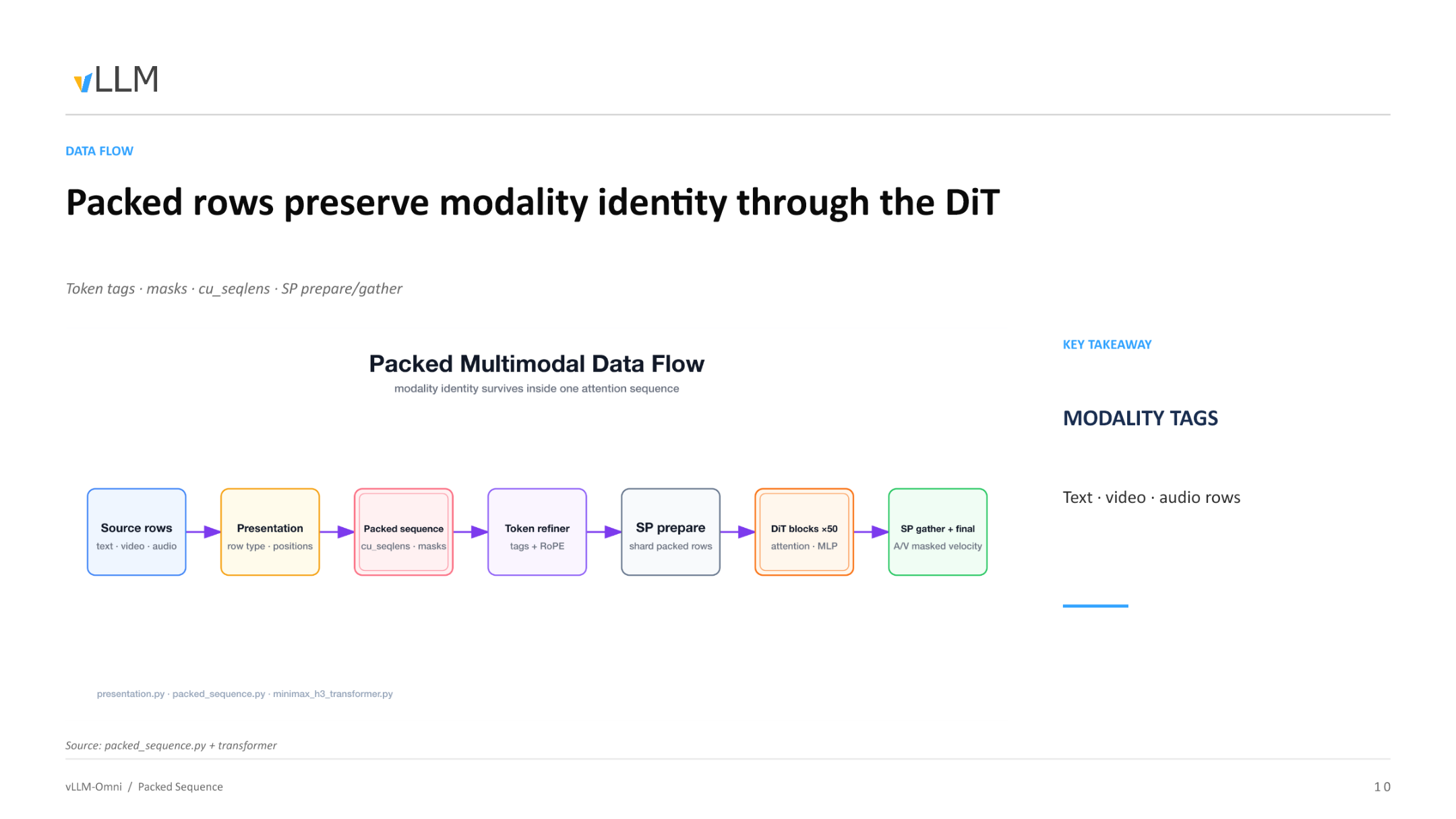Figure: Complete data flow of the packed sequence through the DiT. Source: presentation slides, page 10.

The six stages in the diagram and their key operations:

Stage	Key operation	Metadata added/consumed
Source rows	Group raw text, video, and audio rows by modality	Row type
Presentation	Record modality category and spatial/temporal position for each row	Position indices (positions)
Packed sequence	Concatenate the above rows into a 1D long sequence	Cumulative sequence lengths cu_seqlens, attention masks
Token refiner	Inject modality tags for each token and apply RoPE positional encoding	Tags + RoPE embeddings
SP prepare	Split along the Sequence Parallelism (SP) dimension	Local cu_seqlens per shard
DiT blocks ×50 → SP gather	50 layers of attention + MLP processing, then cross-device aggregation	Output: masked velocity for audio and video

Causal Chain: Why Modality Identity "Survives"

1. Modality tag injection — Each token is assigned a discrete tag (text / video / audio) before entering the DiT. The tag influences the frequency selection of RoPE (Rotary Position Embedding); the positional encoding spaces of different modalities are independent of one another, fundamentally reducing cross-modal positional signal interference.

2. cu_seqlens and masks delineate attention boundaries — cu_seqlens (cumulative sequence lengths) is a 1D integer array recording the start and end offsets of each sub-sequence in the packed sequence. The attention kernel uses this to generate masks, ensuring that tokens within a sub-sequence only perform softmax normalization against tokens belonging to the same sub-sequence.

3. SP prepare / gather preserves boundary consistency — When sequence parallelism splits the long sequence across multiple cards, the splitting logic aligns to cu_seqlens boundaries, preventing a single sub-sequence from being truncated across two cards and causing mask invalidation. After all 50 DiT layers complete, SP gather reassembles the outputs from each shard.

4. Modality separation at the output — The aggregated sequence is still 1D, but cu_seqlens and tags remain queryable at all times. The system slices out each modality's masked velocity accordingly and routes them to the corresponding VAE for decoding.

Minimal Example: How cu_seqlens Marks Boundaries

Suppose a packed sequence contains only two modalities — 10 text tokens (indices 0–9) and 20 video tokens (indices 10–29):

cu_seqlens = [0, 10, 30]

The first sub-sequence covers [0, 10), and the second covers [10, 30). When the attention kernel computes the attention score for token 15 (video), it only performs dot products against keys in the index range 10–29; text tokens at indices 0–9 are masked out, and their weights after softmax are zero.

If 15 audio tokens are added, the array becomes [0, 10, 30, 45], and the three sub-sequences are each self-contained and mutually invisible.

Conclusion

Through modality tags, cu_seqlens, attention masks, and a splitting strategy aligned with sequence parallelism, H3 maintains logical isolation of three modalities within a single physical sequence — from tag injection at the input through masked velocity extraction at the output, all 50 DiT layers never leak across modalities.

Boundary conditions: The presentation materials do not specify the fallback strategy for SP prepare when a single sub-sequence length exceeds the VRAM capacity of a single card, nor do they state whether optional cross-modal attention paths exist between different modalities.

With the data structures clarified, how does this packed multi-modal sequence evolve during the actual denoising loop?

---

4. Joint Audio-Video Denoising Execution Flow

Key question for this section: During the diffusion model's generation process, how do video frames and audio waveforms achieve strict step-by-step synchronization?

Runtime Loop

The diagram below shows the data flow through a single complete denoising step — the core of understanding the audio-video synchronization guarantee.

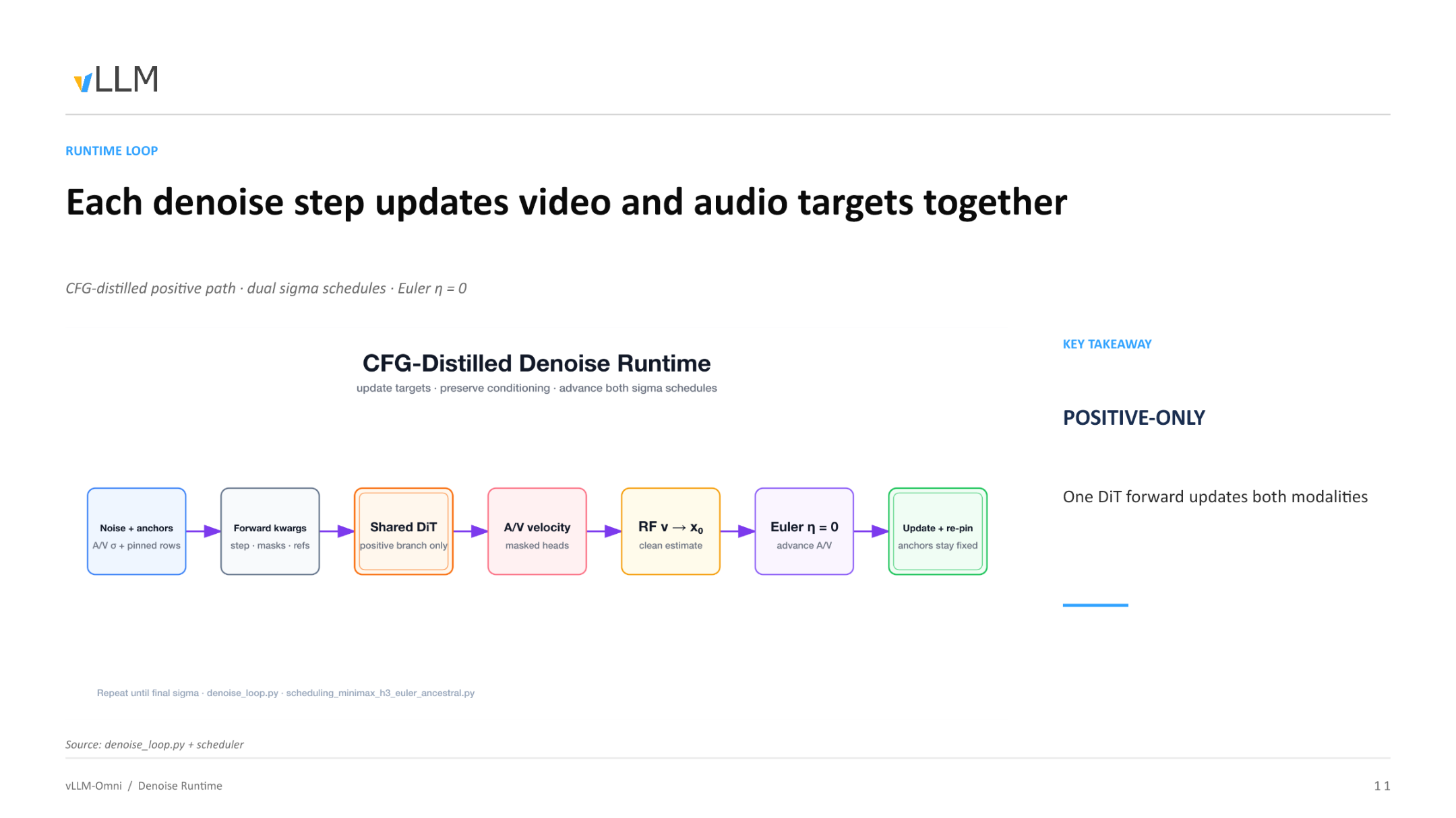Figure: Denoising runtime loop diagram. Source: presentation slides, page 11.

The seven stages in the diagram, explained one by one:

Stage	Node	Function
①	Noise + anchors	Concatenate the current step's audio-video noise state with pinned anchor rows into a unified sequence
②	Forward kwargs	Inject the current step number, modality masks, and reference conditions
③	Shared DiT (positive branch only)	The shared DiT executes only the positive branch; a single forward pass processes both video and audio simultaneously
④	A/V velocity (masked heads)	The output is separated by masked heads into two tensors: video velocity and audio velocity
⑤	RF v → X₀	Use Rectified Flow velocity parameterization to convert the predicted velocity into a clean estimate X₀
⑥	Euler η = 0	A deterministic Euler solver (no additional random noise injected) advances the audio and video states synchronously
⑦	Update + re-pin	Write back the updated audio-video latents; re-pin anchor rows to their original values

The loop starts from the initial σ (maximum noise level), progressively lowers σ toward zero, and strictly repeats the above seven stages at each step.

Key Causal Chains

Why is only one forward pass needed? Conventional CFG (Classifier-Free Guidance) requires separate forward passes for "with text condition" and "without text condition," followed by weighted merging, doubling the compute. H3's DiT has undergone CFG distillation (CFG-distilled), compressing the positive and negative branch behaviors into a single forward path — one forward pass yields predicted velocities for both video and audio simultaneously.

How do dual sigma schedules coexist? Although audio and video share the same DiT, each maintains an independent noise schedule: σ_video(t) and σ_audio(t). The Euler solver at stage ⑥ computes step sizes separately based on each modality's σ value before writing back in unison — this is the key to the two modalities "sharing a model" while "scheduling independently."

Why must anchors be re-pinned? Anchor rows carry known information such as reference frames or reference audio clips. The denoising update attempts to modify all positions in the sequence; therefore, stage ⑦ must restore anchor rows to their original values to prevent reference signals from being overwritten by noise predictions.

State Evolution Example

Using 3 denoising steps as an illustration (the actual step count is 50):

Step 3 (σ_max)
  Pure noise z₃ + anchors → DiT forward → v₃ → Euler(σ₃→σ₂) → z₂ → re-pin

Step 2 (σ_mid)
  z₂ + anchors → DiT forward → v₂ → Euler(σ₂→σ₁) → z₁ → re-pin

Step 1 (σ_min → 0)
  z₁ + anchors → DiT forward → v₁ → Euler(σ₁→0) → x₀ (clean latents)

The final x₀ simultaneously contains the video and audio latents, which are handed to their respective VAEs for decoding into pixel frames and stereo waveforms.

Conclusion

A single DiT forward pass completes the velocity prediction for both modalities, and a deterministic Euler solver advances the audio and video states synchronously within the same time step — this is the fundamental guarantee of absolute synchronization on the physical time axis.

Boundary conditions: η must be 0; introducing random noise would break synchronization through independent random sampling per modality. The re-pin of anchors cannot be omitted; otherwise, the reference signal will degrade across iterations. The presentation materials do not provide specific values for the dual sigma schedule.

The denoising loop design is elegant, but returning to physical reality: the full weights of the 50-layer DiT simply cannot fit into a single GPU. How do we break through the hardware bottleneck?

---

5. Distributed Layerwise Offload (DLO)

Key question for this section: How can a DiT model of approximately 118 GB be run on a VRAM-constrained GPU cluster?

Core Idea: Decoupling Capacity from Residency

The one-sentence essence of DLO (Distributed Layerwise Offload): completely separate "the model's total capacity" from "the amount of data that actually needs to reside in GPU VRAM during computation" — DiT layers not participating in the current computation are offloaded to host CPU memory and streamed back on demand during computation.

The diagram below contrasts the memory layouts of the full-residency baseline and the DLO-optimized scheme, visually demonstrating the source of VRAM savings.

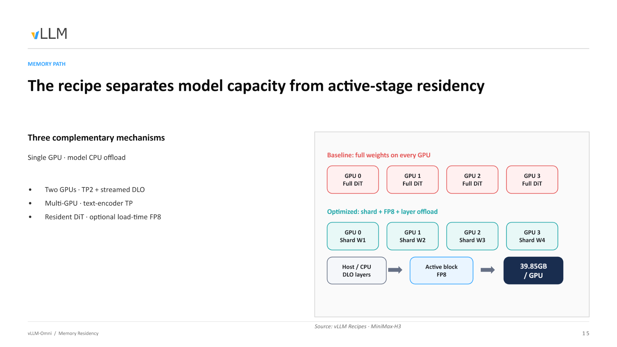Figure: In the Baseline scheme on the left, each GPU holds a full copy of the DiT weights; in the Optimized scheme on the right, weights are sharded and offloaded, reducing per-card VRAM usage to 39.85 GB. Source: presentation slides, page 15.

Key elements in the diagram:

Element	Meaning
GPU 0–3 / Full DiT	Baseline: each card stores a full copy of the weights, leaving very little room for activations
Shard W1–W4	Optimized: weights are split into 4 shards along the tensor parallelism dimension; each card holds only 1/4
Host / CPU — DLO layers	DiT layers not participating in the current computation reside in host DRAM
Active block → FP8	The layer currently being computed is streamed from CPU to GPU, resides at FP8 precision, and is freed upon completion
39.85 GB / GPU	Measured per-card VRAM usage after combining TP2 sharding and FP8 quantization

Execution Flow: A Pipeline of Three CUDA Streams

The DLO runtime relies on three parallel CUDA streams working in concert:

1. Compute Stream — Executes the forward computation of the current DiT layer on the GPU.
2. H2D Stream (Host → Device) — While the compute stream is working, it prefetches the next layer's weights from host DRAM to the GPU.
3. All-gather Stream — In multi-GPU scenarios, each card retrieves its own shard slice from the host, then reassembles the full layer weights via All-gather communication for computation. Once computation completes, the reassembled full weights are immediately discarded.

Causal chain summary: Insufficient VRAM → inactive layers placed in CPU DRAM → H2D stream transfers on demand → multiple cards share the same host memory via All-gather → weights are freed after computation → the GPU always retains only the overhead of one active block.

From Single Card to Multi-Card: Sharing Instead of Replicating

Early single-card CPU offload schemes, when scaled to 8 cards, required maintaining 8 copies of the weights on the host side. The "distributed" in DLO addresses precisely this problem: 8 cards share the same copy of weights on the host, each fetching only its own shard slice. In an 8-card data parallelism scenario, host memory usage is nearly the same as for a single card.

Conclusion

DLO is the survival foundation for VRAM-constrained devices, enabling consumer-grade GPU clusters to run 100 GB-class DiT models. However, it fundamentally trades PCIe bandwidth for VRAM capacity — on a pure PCIe topology, H2D transfer latency may not be fully hidden by the compute stream, limiting throughput. NVLink interconnects can further mask All-gather communication costs; conversely, if the hardware has ample VRAM, full weight residency is the superior choice.

Boundary conditions: 39.85 GB is the value achieved with TP2 and FP8 combined. The presentation materials do not provide end-to-end latency comparison data before and after enabling DLO.

With the VRAM problem addressed, another thorny issue surfaces during computation: the underlying kernel crashes when faced with an irregular sequence length like 58,758.

---

6. Boundary Trimming for Packed Attention

Key question for this section: Why does the underlying attention operator produce non-finite values when processing 58,758 effective tokens?

The Contradiction: Aligned Length ≠ Effective Length

The attention kernel on the GPU requires input sequence lengths to be aligned to a specific block size when allocating shared memory and scheduling thread blocks. The aligned length is 58,816, while only 58,758 tokens actually carry semantics — there are 58 padding tokens between them.

Item	Value
Effective token count	58,758
Aligned length	58,816
Excess padding	58

Causal Chain: How Padding Triggers a Crash

1. Alignment zero-padding — To satisfy the kernel's memory alignment constraint, 58 padding tokens with undefined values are appended to the end of the sequence.
2. Weight contamination — During the softmax normalization stage, the query-key dot products at padding positions are not masked out, and anomalous values are included in the denominator.
3. SAGE overflow — The SAGE operator in TRTLLM (TensorRT-LLM, the default attention backend) encounters the contaminated softmax distribution and produces NaN or Inf.
4. Cascading propagation — Once a layer outputs non-finite values, the residual connections of all subsequent DiT layers amplify the error layer by layer, rendering the generation result completely unusable.

Key insight: The trigger condition is not the presence of padding per se, but that padding is treated as valid tokens and participates in attention computation inside the kernel.

Fix

vLLM-Omni performs a strict boundary trim (Trim Padding) before kernel dispatch: truncating 58,816 precisely back to 58,758, ensuring that only effective tokens enter the operator.

The diagram below shows the position and effect of the trimming operation within the pipeline.

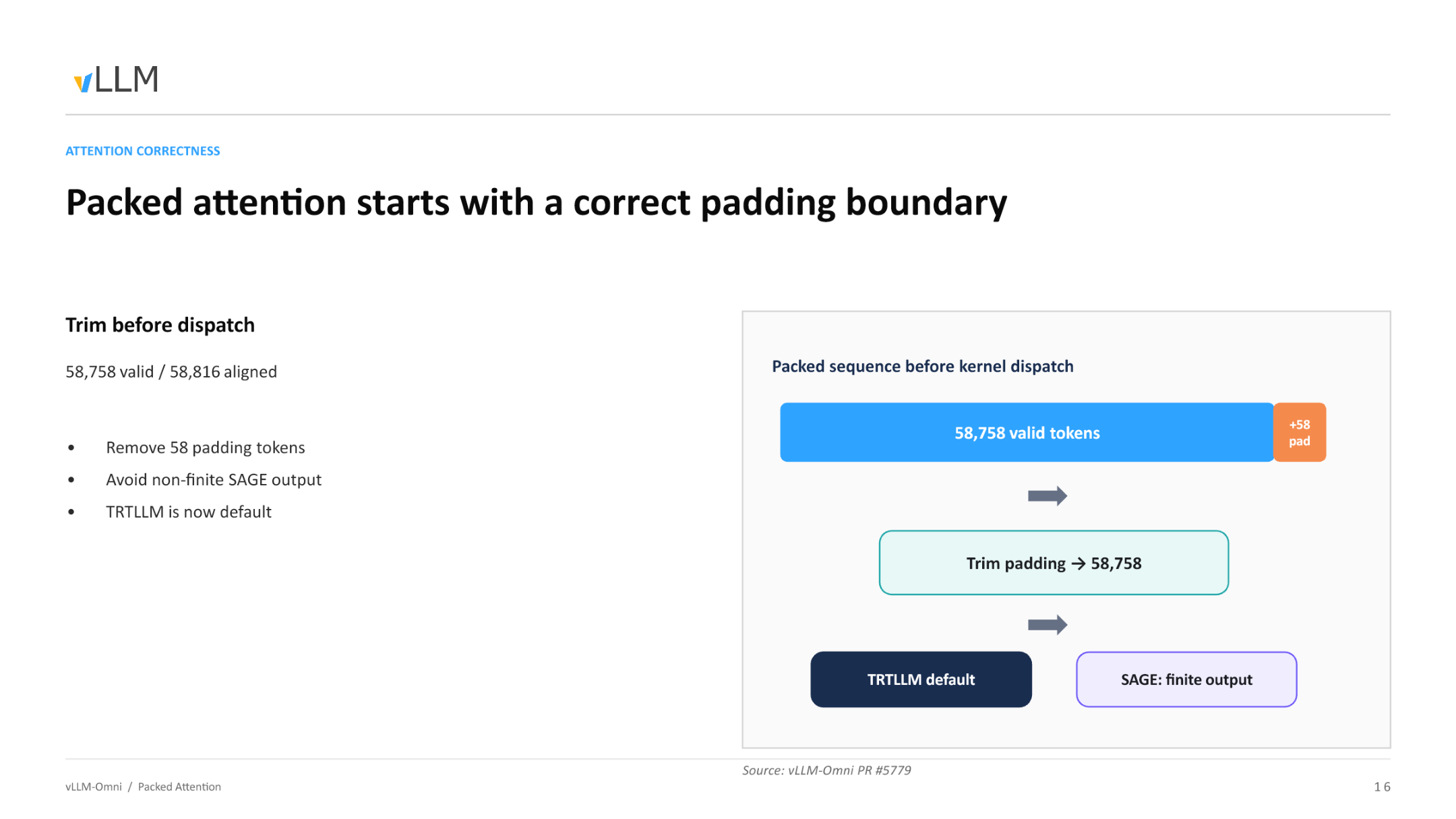Figure: The flow of trimming padding from the packed sequence before kernel dispatch. Source: presentation slides, page 16.

Three stages from left to right in the diagram:

• Left block — "Packed sequence before kernel dispatch," annotated with 58,758 effective tokens and +58 Pad, representing the aligned original state.
• Middle arrow — The "Trim padding → 58,758" operation is executed, physically truncating the 58 excess positions.
• Right result — With TRTLLM as the default backend, the SAGE operator restores numerical correctness (finite output).

The trimming operation itself has negligible overhead — it merely adjusts the length parameter and pointer offset passed to the kernel, with no data copy involved. When the effective token count happens to be an exact multiple of the block size, the padding length is zero, and trimming degenerates into a no-op.

Conclusion

Precise boundary control is the prerequisite for maintaining numerical stability in long-sequence multi-modal kernels. This is an engineering issue that appears trivial but can cause the entire inference pipeline to fail.

Boundary conditions: The presentation materials do not provide alignment granularity details for other block sizes or different GPU models; actual deployments should follow the kernel configuration of the specific TRTLLM version.

With VRAM and operator stability resolved, how can we further squeeze the compute power of high-end GPUs to reduce the long latency imposed by the 50-step loop?

---

7. Step-Level Scheduling and Cross-Step Caching

Key question for this section: On high-end GPUs with ample VRAM, how can compute utilization be maximized and generation time reduced?

The Real Bottleneck on High-End Cards

DLO trades PCIe bandwidth for VRAM capacity. But on high-end compute cards with abundant VRAM, VRAM itself is not scarce; GPU compute speed far exceeds PCIe transfer speed, and the communication overhead introduced by DLO instead creates large compute bubbles, causing inference throughput to decrease rather than increase. Developers confirmed this phenomenon during testing.

Therefore, on such hardware, the optimization direction shifts from "saving VRAM" to two goals: filling idle compute and eliminating unnecessary computation.

Step-Level Scheduling: Making the Denoising Loop Visible to the Scheduler

In traditional diffusion inference, all denoising steps of a request are treated as an indivisible unit — the scheduler can only process the next request after the current one finishes entirely. The core idea of step execution is to expose each step of the denoising loop to the scheduler, making it a schedulable unit. This is a control-plane feature — it does not change the model's computation logic but changes how requests are orchestrated:

Capability	Description
Step-level interleaving	Steps from different requests can form a batch and execute in parallel
Immediate termination	A canceled request can be stopped at the next step boundary
Continuous batching	Enables Continuous Batching for DiT, analogous to autoregressive models

The diagram below shows the interleaving of three requests on a timeline, visually illustrating how step-level scheduling improves compute utilization.

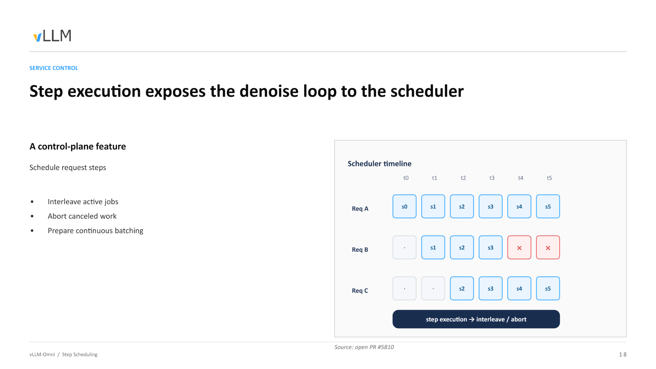Figure: Req A executes continuously from t0 through s0–s5; Req B joins at t1 and executes s1–s3 before being canceled (× mark), with subsequent steps no longer consuming compute; Req C joins at t2 and executes s2–s5. Source: presentation slides, page 18.

Row-by-row explanation:

• Req A arrives first and continuously completes 6 denoising steps starting from t0.
• Req B joins at t1; its s1, s2, s3 are batched together with Req A's corresponding steps and sent to the GPU. After t3, the user cancels this request; the scheduler marks it as terminated at the step boundary of t4, immediately releasing resources. Without step-level scheduling, Req B's remaining steps would still run idle to completion.
• Req C joins at t2 and interleaves with A (and the briefly coexisting B) through t5.

The essence of this interleaving is equivalent to Continuous Batching in LLM inference. This feature is currently being developed as open PR #5810.

Cross-Step Caching: Skipping Redundant Denoising Computation

Step-level scheduling addresses "filling compute"; cross-step caching focuses on "eliminating unnecessary computation."

During the DiT denoising process, intermediate features between adjacent steps are often highly similar. The causal chain of cross-step caching:

1. Observation — The output difference between step s_k and s_k-1 at the DiT layers is very small.
2. Decision — Compute a similarity metric between the two steps; if it falls below a threshold, deem the step "reusable."
3. Execution — Skip the complete DiT layer forward computation for the current step and directly reuse the previous step's result.
4. Benefit — Skipped steps incur near-zero compute overhead, reducing total denoising latency accordingly.

The diagram below shows the comparison between baseline and caching strategies.

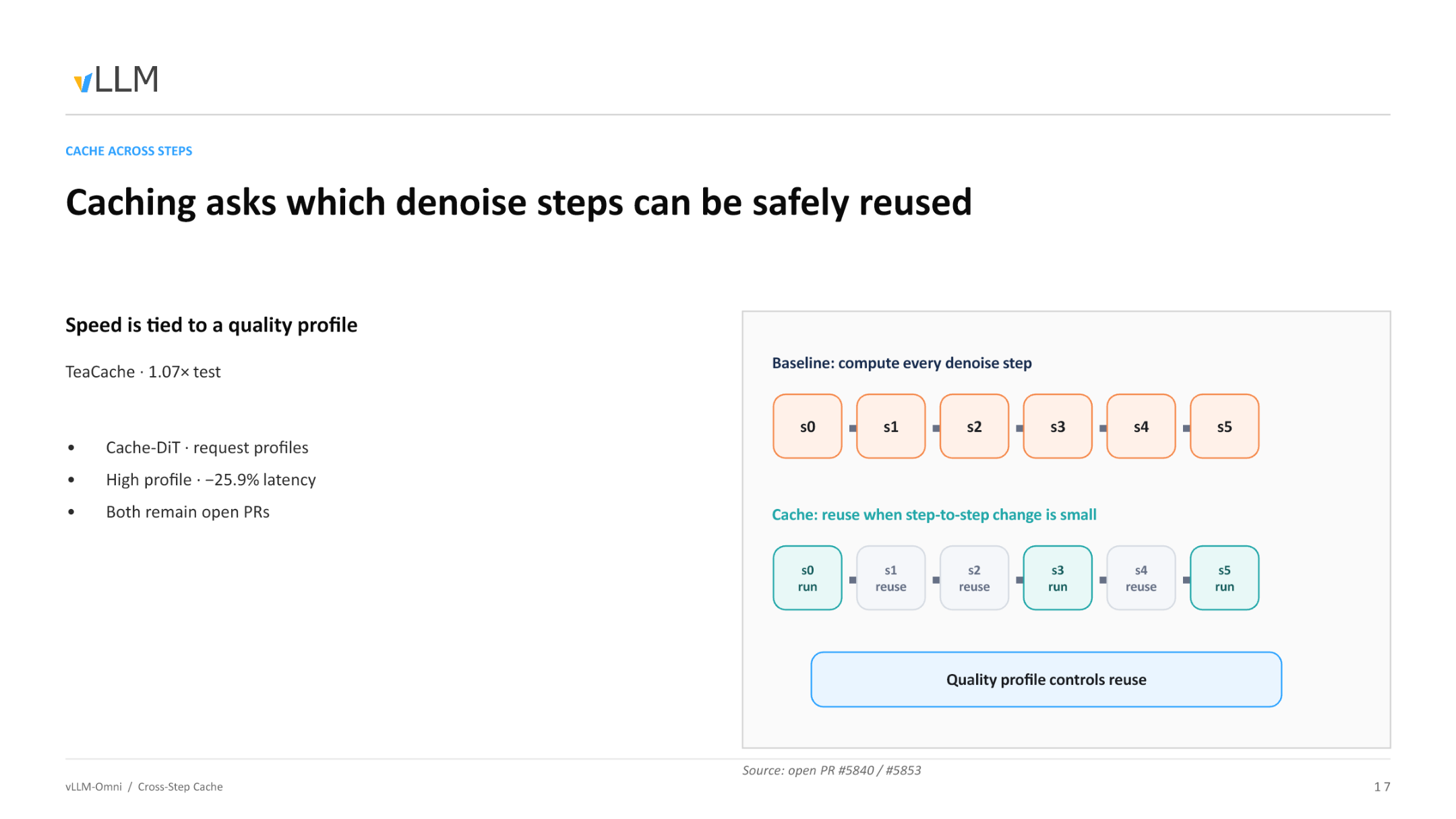Figure: The baseline at the top executes full computation for every step; the caching strategy at the bottom directly reuses results from the previous step for steps with high similarity, reducing actual computation. Source: presentation slides, page 17.

The vLLM-Omni community is currently integrating two cross-step caching algorithms:

Algorithm	Skip granularity	Disclosed performance	Status
TeaCache	Skip entire steps	Test data shows 1.07× speedup	open PR #5840
Cache-DiT	Skip specific layers within a step	25.9% latency reduction at high profile	open PR #5853

The two are not mutually exclusive and operate at different granularities: TeaCache decides "should this step be skipped entirely," while Cache-DiT decides "which layers within this step can be skipped." The 25.9% latency reduction for Cache-DiT corresponds to its high profile setting — the more aggressive the tier, the more skips, the faster the speed, but the greater the generation quality loss.

Conclusion

The optimization core on high-end GPUs lies in hiding latency and reducing unnecessary computation. Step-level scheduling fills compute gaps through request interleaving, while cross-step caching shortens per-request latency by skipping redundant computation. The two can be stacked, but both come with prerequisites — the former requires sufficient concurrent request volume, and the latter requires an explicit trade-off between speed and generation quality.

Boundary conditions: Developers mentioned that step-level scheduling has not yet shown benefits on consumer-grade GPUs; gains are expected to be more pronounced in multi-card high-end cluster scenarios. Both caching techniques are at the open PR stage and have not been merged into the main branch. The presentation materials do not provide specific data for Cache-DiT low/medium profiles.

Once all scheduling and algorithmic optimizations are in place, the final step is landing them on physical clusters and deployment topologies.

---

8. 4-GPU Combined Deployment and Physical Boundaries

Key question for this section: With all optimization techniques combined, how should the production environment be deployed to support all task types through a single API?

Shared Workflow Overview

The diagram below shows the final form of the combined deployment mode, where all previously discussed optimizations converge.

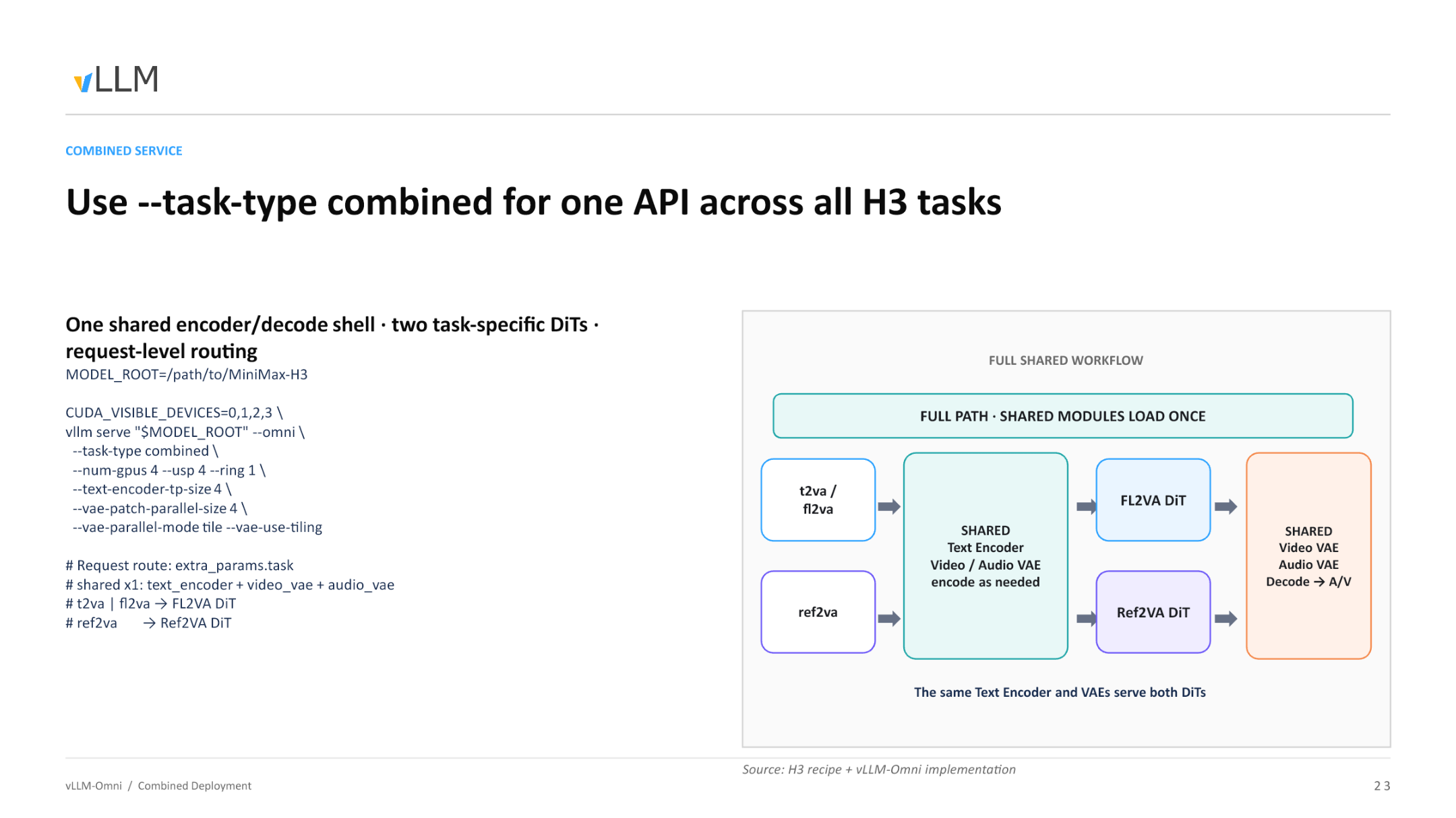Figure: Complete data flow of combined deployment — shared modules are loaded only once, and requests are routed to the corresponding DiT by task type. Source: presentation slides, page 23.

The diagram is divided into three regions from left to right:

Region	Modules included	Load count
Shared encoding shell	Text Encoder (Qwen3-VL, 2B) + Video VAE encoder + Audio VAE encoder	1 time
Task-specific denoising	FL2VA DiT / Ref2VA DiT	1 copy each, routed per request
Shared decoding shell	Video VAE decoder + Audio VAE decoder	1 time

Key observation: Shared modules are loaded only once. In the VRAM of the 4 GPUs, the Text Encoder and dual VAEs each hold a single copy of weights, rather than being redundantly allocated per task.

Launch Parameter Reference

The minimum runnable command given in the presentation materials:

MODEL_ROOT=/path/to/MiniMax-H3

CUDA_VISIBLE_DEVICES=0,1,2,3 \
vllm serve "$MODEL_ROOT" --omni \
  --task-type combined \
  --num-gpus 4 --usp 4 --ring 1 \
  --text-encoder-tp-size 4 \
  --vae-patch-parallel-size 4 \
  --vae-parallel-mode tile --vae-use-tiling

Core parameter breakdown:

• --task-type combined: Enables Combined Serving; a single process simultaneously loads both FL2VA and Ref2VA.
• --num-gpus 4 --usp 4 --ring 1: 4-GPU USP (Unified Sequence Parallelism) with ring dimension set to 1.
• --text-encoder-tp-size 4: Text Encoder uses 4-way tensor parallelism.
• --vae-patch-parallel-size 4 --vae-parallel-mode tile --vae-use-tiling: VAE decoding uses tile-mode patch parallelism; high-resolution frames are sliced and distributed across 4 cards.

Design intent: Ensure that the encoding, denoising, and decoding stages all uniformly utilize all 4 GPUs, preventing one stage from monopolizing a single card while the others sit idle.

Request-Level Routing

The caller specifies the task type via the extra_params.task field in the request body. Routing occurs after shared encoding completes but before DiT denoising begins — different requests can take different pipelines at the same time, with no need to restart the server or switch models.

Physical Boundaries and Engineering Caveats

Combined deployment layers all optimizations onto a single topology, but the layering itself introduces new constraints:

1. DLO may yield negative returns on consumer-grade hardware. When PCIe bandwidth is insufficient, the latency from offload-and-refill may exceed the batching benefit gained from the VRAM it saves. The presentation materials do not provide specific throughput comparison data for consumer-grade hardware; benchmark testing should be conducted prior to deployment.

2. Cross-step caching speedup has a strict trade-off with generation quality. The more aggressive the caching, the more layers skipped, the faster the inference — but at the cost of irreversible quality degradation. In combined mode, the optimal caching thresholds for the FL2VA and Ref2VA pipelines may differ; a uniform configuration risks excessive skipping.

3. Stacking multiple parallelism strategies introduces potential conflicts. Combined deployment simultaneously activates USP (denoising stage), tensor parallelism (encoding stage), and tile-based patch parallelism (VAE stage). The three strategies have different GPU inter-communication requirements — USP relies on all-to-all, tensor parallelism relies on all-reduce, and tile parallelism involves spatial-shard stitching. When the hardware topology is not an ideal NVLink full-mesh, communication contention may become a hidden bottleneck. Several advanced features (e.g., Continuous Batching, DLO, and cross-step caching) are all currently at the open PR stage; enabling them simultaneously may trigger conflicts.

---

Conclusion

1. MiniMax-H3 achieves physics-level synchronized audio-video generation through a shared DiT — a single forward pass simultaneously outputs predicted velocities for video and audio, with a deterministic Euler solver guaranteeing step-by-step alignment — but this also introduces an inference disaster of approximately 118 GB in weights and a 58,758-token long sequence.

2. vLLM-Omni's Combined Serving mode dramatically reduces VRAM redundancy in multi-task concurrency via "shared shell + task routing" — the Text Encoder and dual VAEs remain as singletons, while FL2VA and Ref2VA DiTs are dynamically switched at the request level, avoiding redundant weight loading.

3. Packed sequences maintain logical isolation of multiple modalities through modality tags, cu_seqlens, and attention masks — three modalities coexist in the same physical sequence but are mutually invisible, safeguarding the DiT's correct semantic processing at the data structure level.

4. DLO provides survival headroom for low-VRAM devices — combined with TP2 sharding and FP8 quantization, per-card VRAM can be compressed to 39.85 GB, at the cost of introducing a PCIe bandwidth bottleneck.

5. Step-level scheduling and cross-step caching are the core weapons for squeezing compute power from high-end GPUs — the former achieves Continuous Batching through request interleaving, while the latter reduces latency by skipping redundant denoising steps (25.9% reduction under Cache-DiT high profile) — but both remain at the open PR stage.

6. Precise kernel boundary trimming is a numerical safety prerequisite for long-sequence multi-modal inference — 58 padding tokens are sufficient to cause a NaN crash across the entire inference pipeline and must be strictly truncated before dispatch.

7. Production deployment is fundamentally about finding the optimal solution across VRAM capacity, PCIe bandwidth, generation quality, and inference latency for a specific hardware topology — there is no universally optimal engineering solution, only precise compromises tailored to specific interconnect conditions and business requirements.

Known Limitations

• DLO may yield negative returns on consumer-grade GPUs (PCIe bandwidth–constrained); the presentation materials do not provide throughput comparison data for this scenario.
• The acceleration effect of cross-step caching (TeaCache, Cache-DiT) is strictly coupled with quality degradation; specific data for low/medium profiles has not been disclosed.
• Several advanced features (Continuous Batching PR #5810, TeaCache PR #5840, Cache-DiT PR #5853) have not been merged into the main branch; enabling them simultaneously may trigger conflicts.
• Combined deployment mode requires a specific hardware topology (e.g., 4-card NVLink interconnect) and correct request parameter routing to function properly.
• This analysis is based on presentation slides and transcript materials; certain source code details (e.g., the extra_params.task field name, the specific implementation in PR #720) are marked as pending verification.